
AN ABSTRACT OF THE THESIS OF
Joseph H. Haxel for the degree of Master of Science in Oceanography. Presented
on February 1, 2002. Title: The Sediment Response of a Dissipative Beach
toVariations in Wave Climate.
Abstract Approved:
Robert A. Holman
Using wave and wind data from nearby buoys and gauges, real time
kinematic global positioning system (RTK-GPS) and light detection and ranging
(lidar) topographic survey data, and a robust video record, we have quantified the
Large Scale Coastal Behavior
(LSCB) of a dissipative end member beach in the
Pacific Northwest. This study of Agate Beach from 1992 - 2001 reveals important
observations of beach behavior on temporal and spatial scales that have received
little attention in recent nearshore research. Similarly, the high-energy conditions
characteristic of the Agate Beach study site define it as an dissipative end member
that is not well understood.
In order to describe the variability of the system at spatial scales of
hundreds of meters to kilometers and time scales of months to years, regression
models for wave parameters and the beach sediment response were developed
consisting of annually periodic functions superimposed upon long-term trends. The
Redacted for privacy

amplitudes of the seasonal periodicity in significant wave heights
(AHS = 0.94 m ±
0.06), dominant wave period (At,, = 2.1 sec ± 0.1), and mean wave direction (A8
12.3° ± 2.0) exhibit larger variability than the long-term trends observed within a
year (flH= 6.7 cmIyr±2.6,/3T=O.15 seclyr± 0.04, ,69= 3° SIyr± 1.0).
Agreement between the long-term trends in wave statistics and morphology
suggest a directly forced beach response. Assuming alongshore transport of
sediment at Agate Beach is wave-driven, the long-term increase in significant wave
heights
(PHS)
and change to a more southerly approach in wave direction (3 e),
coincident with the 1997-98 El Niflo/ 1998-99 La Nina sequence, correlate with the
increase in sediments along the beach (AVb =
l.84x105 m3). Predictions of wave-
driven alongshore transport estimate a net accretion at Agate Beach
(er =
2.73x1 08 m3) over the 9 year record length. In addition to the long-term increasing
trend in sediment volume, a seasonally based fluctuation in sediments is observed
(Avb
=
7.85x10⁴ m3
± 2.13x10⁴). Video image analysis shows this increase in
subaerial beach sediment volume at the northern end of the Newport littoral cell
also coincides with the long-term offshore migration of the outer sand bar
(I3oBx =
11.0 mlyr ± 0.8). This result also suggests accretion of sediments in
a wider cross-
shore region than observed in the survey record. Similar to the signature of beach
volume variations, the cross-shore position of the outer sand bar also varies with
season
(AQBX
= 114.9 m ± 4.2). The seasonal migrations in the outer sand bar
position displays much larger variations than the long-term behavior described by
/3OBx

Analysis of 27 topographic surveys resolves the cross-shore structure of the
time varying beach surface. Using empirical orthogonal functions (EOF), 2 distinct
eigen-modes of variance describe the seasonal patterns of sediment behavior at
Agate Beach. The first mode describes 34% of the variance and is related to the
summer growth of a dune field that is limited to elevations above MHW, z = 1.076
m. Analysis of concurrent wind field measurements shows this mode of variance is
well correlated with aeolian processes. The second mode (21% of the variance) is
wave-driven, and corresponds to the seasonal behavior of the beach surface below
MHW. Observations show the MHW elevation serves as a transitional zone
between dune related and wave-driven processes that affect the seasonal evolution
of Agate Beach.

© Copyright by Joseph Henry Haxel
February 1, 2002
All Rights Reserved

The Sediment Response of a Dissipative Beach to Variations
in Wave Climate
by
Joseph H. Haxel
A THESIS
submitted to
Oregon State University
in partial fulfillment of
the requirements for the
degree of
Master of Science
Presented February 1, 2002
Commencement June 2002

Master of Science thesis of Joseph H. Haxel presented on February 1, 2002
Majo(Professor, representing Oceanography
Dean of College of Oceanic and Atmospheric Sciences
Dean of GrakI'ute School
I understand that my thesis will become part of the permanent collection of Oregon
State University libraries. My signature below authorizes release of my thesis to
any reader upon request.
Joseph H.
axel, Author
Redacted for privacy
Redacted for privacy
Redacted for privacy
Redacted for privacy

ACKNOWLEDGEMENTS
The waves, currents, sand, wind and generally the entire beach experience
has been something I have loved since I was a young child. I have never lived far
from the ocean. From countless hours spent in the water I developed a curiousity
for the natural behavior of sand bars and changes in the beach that affected the
quality of surf my friends and I rode at our home breaks. I would like to thank my
advisor, Rob Holman, for giving me the opportunity, freedom and means to study a
subject matter that is so close to my heart. Rob has given me the gift to know how
to let the data tell the story. I would also like to thank him for his patience,
encouragement, and understanding for my unorthodox approach to completing this
degree in the last few months.
I would also like to thank John Stanley for writing codes that were I OX
faster than the ones I developed, but not letting me know about them until I had
taken 2 weeks to develop my own. His technical support, suggestions and jovial
manner are something I will greatly miss. I would also like to thank members of
the CIL, in particular: Chris, for never turning down a chance to do some field
work (even in the snow/dark/rain) and countless hours of discussion and jokes;
Nathaniel, for his development of the survey program, the first year of data, and
help along the way; Hilary, for editorial comments and advice; Walt, for good
stories and help with the argo and jet skis, and all the other people I have come in
contact with throughout the Argus world for their time and insight.

Thanks to my family for their support and words of encouragement. Thank
you Sammie for moving up to Oregon with me and volunteering to serve as the
Coastal Imaging "Lab", and Gus for just being "Goose". And most importantly,
thank you Jesica for believing in me and reminding me to always do what is good
and right. And last but not least, thank you Mother Ocean for blessing us with your
beauty.
This research was funded by the Office of Naval Research grant # N00014-
96-10237.

TABLE OF CONTENTS
Chapter 1:
INTRODUCTION
.
1
Chapter 2:
FIELD SITE AND DATA SOURCES
.................................
5
2.1 Field Site Description
.........................................................
5
2.2 Data Sources
....................................................................
10
2.2.1
Wave and Wind Climate Data
...................................
10
2.2.2
Topographic Data
.................................................
13
2.2.3
Video Data
.........................................................
19
Chapter 3:
DATA ANALYSIS AND RESULTS
..................................
23
3.1 Introduction to Analysis Methods
.........................................
23
3.2 Wave Climate Analysis
......................................................
23
3.3 Wind Climate Analysis
......................................................
43
3.4 Topographic Data Analysis
...................................................
44
3.4.1
Gridding and Transformation
.................................
44
3.4.2
Beach Surface Change Analysis
..............................
51
3.5 Video Data Analysis
..........................................................
68
Chapter 4:
DISCUSSION
...............................................................
75
Chapter 5:
SUMMARY AND CONCLUSION
.....................................
81
REFERENCES
..............................................................................
84

LIST OF FIGURES
Figure
2.1
The location of Agate Beach and the NDBC coastal buoys along the
Oregoncoast
...........................................................................6
2.2
Aerial photograph of Agate Beach taken July 5, 2000 looking southward...7
2.3
NDBC coastal buoys measure II, T and 8 ...................................... 12
2.4
The timeline of topographic surface data collected at Agate Beach
from Argo (RTK-GPS) and lidar based surveys................................
15
2.5
The amphibious Argo and RTK-GPS measurement system
..................
16
2.6
a) A snap shot of Agate Beach from the Argus video imaging
system on top of Yaquina Head. b) A time exposure image from
thesame hour
........................................................................20
2.7
A "daytimef image composed of the daily average of pixel intensity
calculated from the hourly 10 minute time exposures.........................
22
3.1
Daily mean wave climate observations from the Newport (id# 46050)
and Old Newport (id# 46040) offshore buoys
...................................
25
3.2
Time-lagged cross-correlation and extrapolation model fit for
H5
from Newport and CRB buoy data
.............................................
26
3.3
Time-lagged cross-correlation and extrapolation model fit for
0 from Newport and CRB buoy data
.............................................
27
3.4
The combined records of Newport and extrapolated CRB daily
mean observations of
H5
(a), T (b), and 0(c) from buoy data...............
30
3.5
Time-lagged auto correlation and annual model regression fit for H5........
31
3.6
Time-lagged auto-correlation and annual model regression fit for 0........
32
3.7
Monthly averaged (<X(month,yr)>) and the repeated, 12 member
set of monthly ensemble averaged
annual(<Xe(month)>) wave climate
signals (a & c). (b & d), the long term linear trend fit to
<X(month,yr)>
<Xe
(month)> ..................................................
35

LIST OF FIGURES (continued)
Figure
Page
3.8
<Hse(month)>
plotted with the annual periodic regression modelto show
the intra-annual structure in the
I-Is variability
...................................36
3.9
a) Daily estimates of Qi from wave data. b) The low pass filtered
Qijtime series of predicted alongshore sediment transport flux
..............41
3.10
The net annual time series of wave-driven alongshore sediment
transportWannuai ........................................................................
42
3.11
Threshold filtered, monthly averaged wind speed and direction
from an NDBC anemometer fixed 9.4 m above mean sea level on
the south Yaquina Bay jetty
.......................................................
45
3.12
RTK-GPS gridded data and interpolation errors from a topographic
survey of Agate Beach on November 11, 2000 ................................ 47
3.13
The time-averaged beach surface elevation grid over the
complete survey record length
....................................................
49
3.14
The transformation of the mean beach surface from Z to W space
............50
3.15
Statistics of surface variability at Agate Beach over the survey
recordlength
......................................................................... 52
3.16
The number of observations (N) at each grid node over the 27
survey record length ................................................................ 53
3.17
The range in elevation at each grid node calculated by
subtracting the minimum elevation from the maximum elevation
observed throughout the survey time series
......................................
55
3.18
The alongshore averaged statistics of the Agate Beach survey
timeseries
............................................................................ 56
3.19
Statistics of Agate Beach as a function of surface elevation
................... 58
3.20
EOF analysis of the normalized survey record reveals two
distinct modes of surface variability
.............................................
61

LIST OF FIGURES (continued)
Figure
3.21
The dune mode EOF and monthly wind time series correlation.............. 62
3.22
The monthly mean alongshore wind velocity
v,Id
plotted against
the dune mode amplitudes from the 1995-96 survey record.................. 63
3.23
a) A time exposure image of Agate Beach collected by the Argus
station on top of Yaquina Head. The box indicates the study area
covered by the topographic surveys. b) A cross-shore schematic
diagram of the volumetric sediment calculation from equation 15
...........
66
3.24
The demeaned beach volume time series,
Vb,
calculated from
all of the topographic surveys
.....................................................
67
3.25
a) A rectified or plan view of the "daytimext' image from Figure 2.8
in local coordinates. b) The pixel intensity profile corresponding to
each of the cross-shore transects shown in (a)
..................................
69
3.26
The normalized timestacks composed of "daytimex" images from
the 3 cross-shore profiles shown in Figure 3.24
................................. 71
3.27
The "daytimex" timestack history of the cross-shore intensityprofile
aty = 0 m. The cross-shore position of the seaward edge of the
outer sandbar (ob,o) ................................................................ 73
3.28
The alongshore averaged, cross-shore position of the outer sand bar,
OB. and the least squares multiple linear regression fit,
OBxmod,
to the
OBtime series
......................................................................
74

LIST OF TABLES
Table
Page
Comparison of annual wave statistics, beach slopes and Iribarren
#'S
of 3 North American beaches
........................................................
9
2
Contribution of NDBC Oregon coastal buoys for wave climate
records at Agate Beach
..............................................................
11
Dates of Argo and Lidar topographic surveys of Agate Beach
................
14
4
Comparison of model coefficients for wave climate, beach sediment
volume, and outer sand bar position
...............................................
76

LIST OF SYMBOLS
Symbol
long-term linear trend (equation 2)
/3x0
offset for regression fit (equation 2)
A
Vby
the net increase in volume over the topographic survey time
series
ex
unmodeled residuals (equation 2)
phase of the seasonal cycle (equation 2)
elevation skewness with respect to cross-shore position
cross-shore skewness with respect to elevation
gain of the linear regression wave data extrapolation model
(equation 3)
8
wave angle
1
p cross-correlation statistic
standard deviation in elevation with respect to cross-shore
position
standard deviation in cross-shore position with respect to
elevation
Iribarren number
t1annua1
net annual alongshore sediment volume transport from Qi
Y'net
net total alongshore sediment volume transport from Qi
w
frequency of the seasonal cycle (equation 2)

LIST OF SYMBOLS (continued)
Symbol
amplitude of the seasonal cycle (equation 2)
c
wave celerity
C
offset of the linear regression wave data extrapolation model
(equation 3)
D
survey domain in Z space
D *
survey domain
D,
transformed to W space
E
wave energy
Eresx unmodeled residuals (equation 3)
g gravitational acceleration constant
h
water depth
H significant wave height
I
video image pixel intensity
alongshore immersed-weight transport rate
K
dimensionless constant
deep water wave length
LSCB
Large Scale Coastal Behavior
n
ratio between wave group and phase velocity
N*
effective degrees of freedom
cross-shore position of the outer sand bar with respect to
alongshore location
OB
alongshore mean, cross-shore position of the outer sand bar

Symbol
OB10d
F!
QI
Qi
Q
Qy
r0
rexi
S
sxy
Uand V
LIST OF SYMBOLS
(continued)
regression model of OB time series using equation 2
alongshore component of wave power
alongshore volume transport rate predicted from wave data
low-pass filtered
Qi
time series
cross-shore sedimet flux from survey data
alongshore sediment flux from survey data
alongshore and cross-shore sediment flux from survey data
radius of the circle fit to the time averaged 1 m elevation
contour
extended circle radius to fit entire survey domain
beach slope
alongshore component of onshore radiation stress
dominant wave period
video image pixel coordinates
critical wind velocity threshold to transport Agate Beach
sands
monthly mean alongshore wind velocity from threshold
limited record
observed volume of sediment in survey region
regression model of
Vb
time series using equation 2
complex space where alongshore curvature from Z space is
removed

LIST OF SYMBOLS (continued)
Symbol
x
offshore increasing, cross-shore direction in local
coordinates
x'
offshore increasing, cross-shore direction in transformed W
space
<Xe
(month)>
12 member set of ensemble-averaged monthly statistics
<X(month,yr)>
monthly averaged statistics
y
alongshore direction in local coordinates
alongshore direction in transformed W space
z
elevation with respect to NGVD29
Z
complex space defined in local x andy coordinates

THE SEDIMENT RESPONSE OF A DISSIPATIVE BEACH TO
VARIATIONS IN WAVE CLIMATE
Chapter 1 INTRODUCTION
As sea level rises, the threat of coastal erosion has become an increasing
concern to beachfront developers, property owners and coastal planners. Beach
erosion events strip large volumes of sand from the beach face, and transport it
offshore and alongshore on varying spatial scales. While one area of a beach is hit
hard by the onset of storm waves and loses the majority of sand on its beach face,
another region of the beach, sometimes only a few kilometers away may experience
little loss. Alternatively, during calmer months, certain areas of the beach may
experience larger amounts of accretion. These fluctuations in the volume of sand
along a beach affect its ability to serve as a dissipative buffer in protecting valuable
property from the attack of high-energy storm waves. An understanding of the
behavior of beaches on a variety of temporal and spatial scales is required to make
accurate model predictions of the sediment response to both short and long-term
variations in forcing.
Beach erosion events are episodic in nature and well correlated with the
arrival of high-energy storms at the coastline. Modern nearshore science has
focused on processes involving short-term beach variability at time scales of
seconds to weeks and length scales of centimeters to hundreds of meters.
Observations of short-term beach and sand bar behavior are based on short, intense

2
field experiments (Sallenger et al., 1985; Gallagher et al., 1998, Plant and Holman,
in review). These types of studies of beach and sand bar behavior have improved
the knowledge base as well as the performance of process based models in
describing the short-term morphologic evolution of beaches.
Despite the improvements in short-term (seconds to weeks) process models
of sediment transport and morphologic change, when integrated through time, these
models produce results that are generally thought to be unrealistic (Stive et al.,
1995, De Vriend, 1997). As process based models are stepped through longer time
intervals, non-linear interactions between the morphology and fluids are often not
accounted for and may create instabilities within the long-term evolution of the
system.
In addition to the episodic erosion of beaches caused by single storm wave
events, longer-term seasonal variability in beach and sand bar behavior may be
introduced by the succession of storm arrivals during the winter (van Enckevort,
2001). Monthly changes in morphology and beach profiles have been correlated
with seasonal changes in wave climate (Winant et al.,1975; Aubrey, 1979 & 1983).
As wave heights increase, winter profiles are defined by a shallow beach slope and
intertidal bar. Conversely, as wave heights subside, summer profiles are marked by
a steeper beach with the bar welded to the shoreline. The cross-shore position of
the offshore sand bars is an important indicator for seasonal beach profile changes
brought on by variations in the wave climate. Birkemeier (1984) also linked the
onshore! offshore migration of offshore sand bars to seasonal changes in forcing.

The seasonal changes in cross-shore profile and offshore! onshore sand bar
migration indicate a seasonal cross-shore sediment transport pattern. Estimates of
the seasonal cross-shore flux of sediments along beaches have hardly been
quantified.
The variability of beaches and sand bars on longer temporal and spatial
scales, termed Large Scale Coastal Behavior
(LSCB),
is not well understood. The
behavior of beaches on the scale of years to decades and kilometers has received
less attention than process based studies. The few long-term data sets that are
available reveal unexpected behavior (Plant, et al., 1999, Wijnberg and Terwindt,
1995, Ruessink and Terwindt, 2000). Along several coastlines, a nearly decadal
cycle of bar generation near the shoreline, migration offshore, and subsequent bar
degeneration offshore has been documented. In these studies, this cycle has not
been related to similar variations in the wave climate. Instead, the behavior seems
to be linked to non-linear feedback interactions between the bars themselves
(Ruessink and Terwindt, 2000).
The variability of beaches at LSCB
scales is generally attributed to one of
direct forcing, nonlinearities in direct forcing, nonlinear feedback mechanisms or
some combination of these (Holman and Lippman, 1998). The first two of these
possible mechanisms for beach variability are related to changes in the forcing
(winds, waves, currents, etc.) and are therefore termed a forced response. For
example, the seasonal beach profiles related to winter and summer wave climate
conditions outlined above can be called a forced response. The third form is known

as free behavior since it is the result of instabilities caused by feedback between the
morphology and fluids within the system. The yearly to decadal birth, offshore
migration and degeneration cycle of the sand bars discussed earlier are most likely
manifestations of free behavior.
In this study, wave climate variability is correlated to the forced sediment
response of a beach system in the Pacific Northwest. Large changes in wave
direction coupled with increased wave heights along the Pacific Northwest coast
combined to produce northward transport of beach sediments. A predictive
equation for alongshore sediment transport based on wave driven currents is
compared to field data. Similarly, cross-shore and alongshore sediment fluxes are
quantified using estimates made from topographic beach survey data.
The high-energy nature, low slopes and rugged conditions of Pacific
Northwest beaches makes them dissipative end members that have received little
attention in nearshore research. Using buoy and wind data, topographic survey
measurements and video morphologic analyses, this study quantifies the long-term
and annual behavior of Agate Beach in response to long-term and annual variations
in wind and wave forcing. Patterns of topographic beach surface variability
document where, when, and how the beach surface responds to seasonal changes in
the wind and wave climates, as well as long-term variations brought on by El Niño
and La Nifla ocean conditions.

5
Chapter 2
FIELD SITE AND DATA SOURCES
2.1 Field Site Description
The Oregon coastline is divided into a series of sandy beaches bounded by
basaltic headlands. The continuous stretches of beach between headlands are
known as littoral cells, and are believed to be closed systems with respect to the
volumes of beach sediments they contain (Komar, 1997). Agate Beach is located at
the northern terminus of the Newport littoral cell on the central Oregon coast
(Figure 2.1). The Newport littoral cell extends along 42 km of coastline, bounded
by Yaquina Head to the north, and Cape Perpetua to the south. Two westward
extending rock jetties stabilize the entrance to Yaquina Bay and further divide the
Newport littoral cell into sub-cells. The 5 km long northern sub-cell runs from the
north Yaquina Bay jetty up to Yaquina Head (Figure 2.2). Agate Beach is the 2.5
km stretch of sand within the sub-cell, extending from the southern face of Yaquina
Head to the rocks at the northern end of Nye Beach.
Alongshore curvature of Agate Beach forces directional adjustments of
breaking waves due to refractive processes. Another important aspect of the study
site is the shadowing effect of Yaquina Head on the northern section of Agate
Beach. Swells approaching from a northwesterly direction are partially blocked or
refracted by the large headland that extends 1.5 km from shore. Therefore, the
largest portion of wave energy from northwest swells impacts the southern section
ri
0
C)
C)
C)
0)
46.5
CRB Buoy
46
C)
I
(I)
E
45.5k
Co
I
0
I (_)
C)
I
J
I
z
I
0
o
451
0)
L
New
0
'144.51
aquina Head
Yaquina
-125 -124.5 -124
-123.5
44' I
I
Bay
°W Longitude
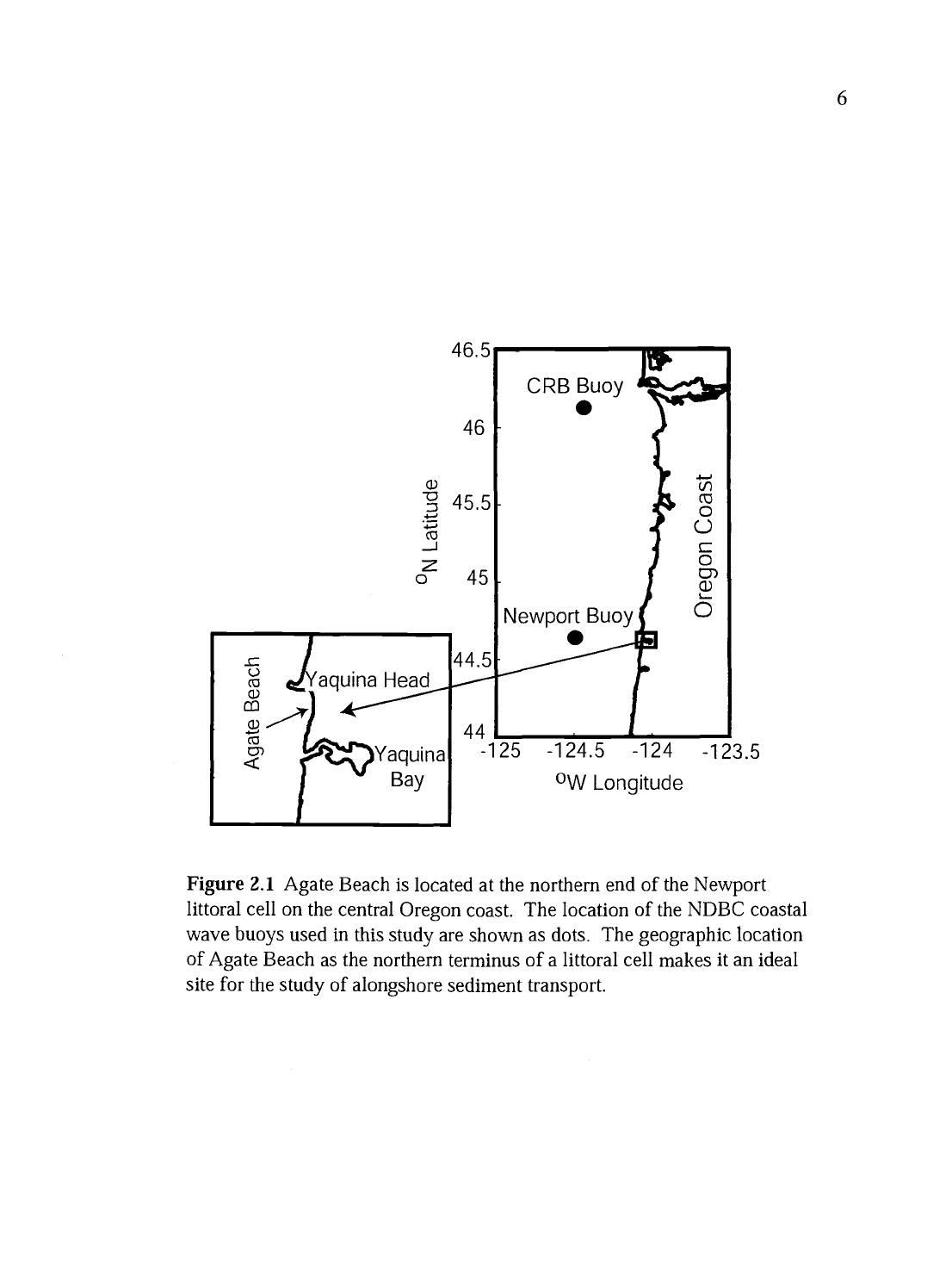
Figure 2.1 Agate Beach is located at the northern end of the Newport
littoral cell on the central Oregon coast. The location of the NDBC coastal
wave buoys used in this study are shown as dots. The geographic location
of Agate Beach as the northern terminus of a littoral cell makes it an ideal
site for the study of alongshore sediment transport.

Yaquina Bay Entrance
N
p
7
Figure 2.2 Aerial photograph of Agate Beach taken July 5, 2000 looking
southward. Note the alongshore curvature of the beach, as well as the northward
bend in Big Creek.

of Agate Beach. Aside from its slight alongshore curvature, Agate Beach generally
faces west allowing full exposure to most of the high-energy storms and swells
generated in the North Pacific Ocean. A small offshore reef in 12 m water depth
roughly 1.5 km from shore offers little protection from the continuous attack of
winter storms.
The sediments at Agate Beach are medium-grained sand, composed mostly
/
ofquartz and feldspar with median grain diameters around 0.2 mm (Ruggiero,
1997). The beach slopes gradually 0(0.01) and is exposed to large semi-diurnal
tides ranging from 2-3 m. At lower tidal elevations there may be up to 600 m of
exposed, subaerial, cross-shore beach surface. Because of its gradual slope, during
large winter storms the surf zone may span up to 1 km as breaking waves dissipate
their energy across the offshore sand bars.
When compared with the incident wave energy impacting other North
American beaches, Agate Beach stands out as a high-energy end member (Table 1).
Comparing the Iribarren numbers
(4)
S
(la)
L
=g7/
/2,r
(ib)
of three representative beaches from the U.S. coastline further reveals the
dissipative nature of Agate Beach defined within the morphologic framework of
Wright and Short (1983). The large waves and low sloping characteristics of Agate

Beach place it well within Wright and Short's (1983) dissipative end member
criterion (
<0.3).
Table 1 Comparison of annual wave statistics, beach slopes and Iribarren numbers
of 3 representative North American beaches (* statistics from this study; tfrom
Guza and Thornton, 1981;
from Birkemeier, 1985)
Site
H5
(m) T (sec) S
Agate Beach,
OR*
2.33
10.6
0.01 0.09
Torrey Pines,
CAt________
1.10 12
0.02 0.29
Duck, NC
0.89 8.8 0.05 0.58
During a normal year, the net alongshore transport of sediment from wave-
driven currents within the Oregon littoral cells is expected to be zero (Komar,
1 998a). Winter waves arriving from the southwest generate northward alongshore
flows that tend to deposit sediment on Agate Beach as the flow encounters the
headland. Conversely, summer waves coming from the northwest drive southward
alongshore flows that strip sediments away from Agate Beach and deposit them
further south within the littoral sub-cell. During El Niño years, the winter pattern is
strengthened by not only a higher frequency of storm wave occurrences, but also
larger storm waves arriving from a southerly direction (Komar, 1986). Therefore,

10
during El Niño events, Agate Beach experiences
an accumulation of sediment
resulting from strong northward flows.
Oregon coast weather has a prominent effect on the seasonal evolution of
Agate Beach. During winter months, an onslaught of intense southerly winds and
driving rains batter the coastline, while the
summer is characterized by drier,
warmer air temperatures and northwesterly winds (Komar, 1997). One result of
this seasonal pattern is variation in the impact of two creeks (Big Creek and Little
Creek; Figure 2.2) that cross the beach. During periods of intense rainfall in the
winter, these creeks cut down and wash
upper beach sediments into the inner surf
and swash zone creating offshore deltas (Ruggiero, 1997). Conversely, in
summer
the precipitation is at a minimum, and the
upper beach sediments dry out from lack
of rain and swash infiltration. Strong northwesterly
summer winds then generate a
seasonal dune field in the backshore (Figure 2.2). At their seasonal peak in
September, some dunes reach heights of nearly 2 m and the field
may encompass
50,000 m2. Later in the fall when the wave energy increases, the sand in these dune
fields is recovered by the swash and returned offshore.
2.2 Data Sources
2.2.1
Wave and Wind Climate Data
Wave climate data has been collected by NOAA's National Data Buoy
Center (NDBC) in Oregon's offshore coastal waters near Agate Beach since 1987.

11
The wave record used in this study is compiled from observations collected by
three coastal buoys (Table 2). The Newport buoy is located -30 km WSW of Agate
Beach while the Columbia River Bar (CRB) buoy is located -170 km NW of the
study site (Figure 2.1). The old Newport buoy was located 2 km north of the
present day Newport buoy position, making any measurement differences
negligible for the purpose of this study.
Table 2
Contribution of NDBC Oregon coastal buoys for wave climate records at
Agate Beach
Old Newport
(#46040)
Newport (#46050)
CRB (#46029)
05/28/87 - 11/11/91
11/12/91 - 08/31/00
Filling gaps in Newport
record 11/12/91-08/31/00
The NDBC buoys deployed in Oregon's offshore coastal waters provide
measurements of significant wave heights
(He),
peak spectral periods (7), and
mean wave directions (G) (Figure 2.3). The buoys are moored in 130 m water
depths, roughly 15 km from shore. Each of the wave parameters is sampled for 20
minutes at the start of every hour throughout the day. Significant wave height
(Ha)
is recorded as the average of the upper 1/3 of the measured waves within the
sampling period (http://www.NDBC.noaa.gov/). Dominant period (Tn) is measured
as the peak in the wave energy spectrum, and 9 is evaluated as the mean wave

12
Figure 2.3 The NDBC offshore buoys measure H, T and 0 for 20
minute intervals every hour. The Newport and CRB buoys are
moored in 130 m water depths in Oregons offshore coastal waters.

13
direction associated with the dominant spectral peak. This information provides a
description of the wave climate at Agate Beach over the last 13 years. A NOAA
based tidal gauge (#9435380) in Yaquina Bay also provides tide level observations
referenced to NGVD29 for the Agate Beach area.
Concurrent wind measurements from an NDBC gauge located on the south
Yaquina Bay jetty provide a description of the wind forcing at Agate Beach. The
NDBC anemometer is mounted on a tower 9.4 m above mean sea level roughly 3
km south of the study site. Values for wind velocity and wind direction are
calculated and recorded from 2 minute averaging intervals at the top of every hour.
2.2.2 Topographic Data
The recent advances in survey technology based on global positioning
systems (OPS) have allowed for the dense and accurate coverage of large spatial
areas (Morton et al., 1993; Dail et al., 2000; Plant and Holman, in review). In the
past, covering these large areas of beach with high sampling density over short time
intervals was unimaginable using traditional optical surveying methods. In
addition to the advantages in surveying speed, real time kinematic global
positioning system (RTK-GPS) based techniques provide more accurate position
estimates than traditional optical tracking techniques (Plant and Holman, in
review).
Two RTK-GPS beach survey series were carried out collecting topographic
data of Agate Beach in 1995-96 and 2000-0 1 (Table 3 and Figure 2.4). These

14
Table 3 Dates of Argo and Lidar topographic surveys of Agate Beach
RTK-GPS survey series
#11995 - 1996
Lidar surveys
1997 - 1998
RTK-GPS survey series
#2 2000
- 2001
06-14-95
10-17-97 05-25-00
06-28-95
04-24-98
06-21-00
07-12-95
07-19-00
07-27-95
08-29-00
08-10-95
09-26-00
08-25-95
11-13-00
09-08-95
12-11-00
09-29-95
01-09-01
10-27-95
02-05-01
12-09-95
01-05-96
02-17-96
03-16-96
04-20-96
05-18-96
06-15-96
surveys were undertaken using an RTK-GPS mounted on a six wheel, amphibious,
all terrain vehicle known as the Argo (Figure 2.5), enabling quick and accurate
elevation measurements of the subaerial beach surface during low tide intervals.
By sampling during spring low tide conditions (often in the dark), these surveys
cover the greatest possible cross-shore extent of subaerial beach surface during
each month. Each survey covers roughly 400 m in the cross-shore and 2.5 km in
the alongshore. Sampling at 5 Hz, the current data collection system is capable of
making accurate measurements at vehicle speeds up to 10 mIs. The beach surveys

15
I
I
I I
I
I
I
Argo
* lidar
..
* *
S..
SSS
I
I I
I
I I
1995
1996 1997
1998
1999
2000 2001
Figure 2.4 The time history of topographic surface data collected at Agate Beach
from Argo (RTK-GPS) and lidar based surveys.

16
radio transmitter
GPS rover antenna
Figure 2.5 The RTKGPS collection system. The top panel shows the base station
unit and radio transmitter antenna along with the rover GPS unit mounted on the
Argo. Topographic estimates can be collected at vehicle speeds up to 10 mIs. The
amphibious nature of the Argo makes it possible to measure the beach surface
through creek beds and incoming swash.

17
from series #2 are composed of more than 40,000 elevation measurements
collected in time intervals of 2.5 hours.
The RTK-GPS collection system employed in this study is similar to that
used by Plant and Holman (in review). The survey grade GPS equipment consists
of a base station with a known position, a GPS rover unit mounted on the Argo
(Figure 2.5), and a high powered radio transmitter and receiver. The base station
and rover units (Trimble 7400) collect simultaneous range measurements from a
common group of satellites. The base station compares a measured position with
its known reference position and sends an error correction to the rover unit via the
high-power radio transmitter. The real time kinematic correction supplied by the
base station allows for rover estimates with errors 0(3cm) in the horizontal and
0(5cm) in the vertical. The position measurements made by the RTK-GPS system
are logged on a Fieldworks Inc. computer running Trimble's Hypack software. To
correct for antenna height, the elevation of the RTK-GPS rover antenna mounted
on the Argo is measured during each survey and subtracted from all beach surface
observations.
In October 1997 and April 1998 a collaborative effort between the National
Aeronautic and Space Administration (NASA), the National Oceanic and
Atmospheric Administration (NOAA), and the United States Geological Survey
(USGS) collected topographic data along the California, Oregon, and Washington
coasts in order to capture changes resulting from a strong El Niño event. Using
lidar (light detection and ranging) technology, airborne surveys made surface

18
elevation measurements of the Oregon coastline, including the study area at Agate
Beach. Lidar is a remote sensing, laser-based technology capable of collecting vast
amounts of densely sampled topographic data in short time intervals (Sallenger et
al.,1999). The system collects 3,000 to 5,000 surface elevation shots per second,
yielding roughly 600,000 survey points within the Agate Beach study area for each
survey date. The estimated vertical accuracy of the system is 15 cm (Sallenger, et
al., in review). This data, supplied by the NOAA Coastal Services Center,
supplements the temporal gap in the survey record between the 1996 and 2001
RTK-GPS survey series. By combining the RTK-GPS and lidar data, this study
focuses on topographic changes across 27 surveys spanning 6 years at Agate
Beach.
The topographic data are transformed with a rotation and translation into the
local right hand coordinate system common to the video data with x increasing
offshore. During each survey operation, local control points are collected and their
position is used to calculate the transformation of all the survey observations into
the local coordinate system. All elevations reported are referenced to the National
Geodetic Vertical Datum (1929). Due to the low sloping nature of Agate Beach,
and small footprint of the Argo, elevation errors resulting from the Argo tilt were
small (within the RTK-GPS instrument error) and therefore neglected (Plant and
Holman, in review).

19
2.2.3 Video Data
The powerful waves, extensive surf zone, and strong currents associated
with the dissipative conditions at Agate Beach make it difficult to collect
continuous, in situ measurements of geophysical variables (i.e. currents, waves,
subaqueous profiles). An Argus video imaging system was installed in 1992 by the
Coastal Imaging Lab on top of Yaquina Head to study nearshore processes (Figure
2.2). The accumulated video data set provides ideal temporal and spatial coverage
of offshore sand bar locations. Remote sensing techniques based on these video
images are used to characterize the sediment transport patterns and the morphologic
evolution of the offshore sandbars along Agate Beach.
A snap shot of Agate Beach (Figure 2.6a) from the video imaging system
on top of Yaquina Head captures breaking waves as intermittent patches of white
foam. A time exposure image with the same field of view is created every hour.
Time exposure images are sampled at 1 Hz and are computed as the time-averaged
intensity at each pixel over a 10 minute period. These images resolve the spatial
location of preferential wave breaking indicated by smoothed, bright bands of pixel
intensity (Figure 2.6b). The bright bands of intensity correspond to the locations of
shallow bathymetric features such as sandbars and the shoreline (Holman and
Lippmann, 1987). Time exposure images of Agate Beach have been collected
hourly since 1992. To reduce the data set for this analysis, we use "daytimex"
images composed of the mean pixel intensity from each time exposure image
within a day (Konicki and Holman, 2000). These images have the advantage of

50
100
150
200
250
>
300
350
400
450
0
50
100
150
1
200
250
>
300
350
400
450
0
(a)
(b)
100
200
300
400
500 600
100 200
300
400
500
600
U (pixels)
Figure 2.6 a) A snap shot of Agate Beach from the Argus video imaging
system on top of Yaquina Head. b) A time exposure image from the same hour.
Time exposure images consist of the time averaged pixel intensity over a 10
minute period sampled at 1 Hz. Note the continuous white bands of foam
indicating the position of the offshore sand bars.

21
merging image features that were only visible during certain tidal conditions.
Because they are composed of a continuum of images spanning the daily tidal
cycles, these "daytimex" images capture the shoreline at high tide as well as
sandbars that are only revealed through wave breaking during lower tidal
conditions (Figure 2.7). A total of 3128 "daytimex' images from June 5, 1992
through March 3, 2001 provide a time series for daily estimates of the outer sand
bar location.

22
50
100
150
C,,
200
250
300
350
400
450
U (pixels)
Figure 2.7 A daytimex' image composed of the daily average of pixel
intensity calculated from the hourly 10 minute time exposures. These images
have the advantage of spanning the tidal conditions and therefore give a
representative estimate of wave breaking patterns throughout the tidal cycles.

23
Chapter 3 DATA ANALYSIS AND RESULTS
3.1 Introduction to Analysis Methods
To uncover the relationship between the temporal and spatial sediment
response of Agate Beach to the changes in wave and wind climates, we compare
regression model coefficients produced from variations in H, T, 9, the beach
volume measured from topography
(Vb),
and the cross-shore position of the outer
sand bar (OB). Each of these parameters is modeled as the sum of a periodic
annual signal superimposed upon a long- term trend (2).
X(t)
= A cos(cot+ cb) +/3t+ fl0 +
(2)
In equation 2,
Xrepresents the time series of the modeled variable. The
Acos(at+ çi) term represents the periodic annual signal, while /3,t describes the
longer-term behavior of the time series.
/3x0
is an offset, and c indicates the
unmodeled residual variability within the record. Using the information obtained
from regression model fits to these data, we construct a useful quantification of the
seasonal and
LSCB
of the Agate Beach system.
3.2 Wave Climate Analysis
Breaking waves in the nearshore produce the turbulent energy required to
suspend beach sediments within the water column, which are then advected in the

cross-shore and alongshore directions by currents and other low frequency flows.
The magnitudes and directions of these low frequency flows are largely governed
by the directions and intensities of the incident wave energy (Thornton and
Guza,1986; Komar and Oltman-Shay,1990). In this study we focus on the incident
wave energy band as a means to characterize the general wave climate associated
with nearshore sediment transport along Agate Beach.
Daily mean values for H, T, and Gare calculated from the hourly
measurements made by the NDBC buoys described in section 2.2.1. The wave
directions are adjusted to a local right-hand coordinate system (positive
x
increasing offshore) associated with
00
normal incidence at the center of alongshore
curvature of Agate Beach. Within the local coordinate system, negative incident
angles correspond to waves approaching from the north. The daily mean values for
the combined Newport buoy stations are shown in Figure 3.1. Unfortunately, there
are significant gaps within the Newport record, particularly with regard to wave
direction.
To produce a longer, more continuous time series of wave statistics, the
CRB buoy data is extrapolated to the Newport region by a linear model.
Newp)(t)_ FxXc)(t)+
C
(3)
X represents the wave climate variable. Fx and C represent the gain and offset of
the least squares regression model. The regression analysis reveals an offset in
I-Is
and 8 between the CRB and Newport records (Figure 3.2 & 3.3). The extrapolation

10
c,)5
O
2
2
E1
Old Newport Buoy
Newport Buoy
7 88 89 90 91 92 93 94 9 96 97 98 99 00 (1
I
I I
N
0
----------
0
5Q.
s
87 88
89 90
91 92
25
1
1
93
94 95
96
97 98
99
00
01
time (yr)
Figure 3.1 Daily mean wave climate observations from the Newport (id#
46050) and Old Newport (id# 46040) offshore buoys. Notice the annual cycle in
each parameter as well as some of the large gaps in the record, particularly with
respect to 0.

(a)
CRB
..Nevp.
LJ&1Jt)
92 93 94 95 96 97 98 99 00
time (yr)
(c)
I
Newp
- - model
time (yr)
26
(b)
1
0
Pxy(t)
Pcrjt(95%)
0
500
lags (days)
(d)
95 96 97 989900
time (yr)
Figure 3.2 Time-lagged cross-correlation and extrapolation model fit for H5
from Newport and CRB buoy data. a) The Newport and CRB daily mean 11s
observations during times the records overlap. b) Time-lagged cross-
correlation between the CRB and Newport records. c) The least squares linear
model used to extrapolate the CRB
H5values to the Newport area where gaps
in the record exist. d) The residuals (Erj-j), calculated by subtracting the
model results from the Newport data.

(a)
E
1
I
Ill
I'
'lJ
I[
!It
1
Newp
92 93 94 95 96 97 98 99 00
time (yr)
(c)
0
0
0
i
J1
- model
Newp
92 93 94 95 96 97 98 99 00
time (yr)
C
(b)
1
0.5
a-
[SI
-0.5
5
-40
-60
27
- Pxy(t)
.-_p
.(95%)
crit
0 50
lags (iays)
(d)
92 93 94 95 96 97 98 99 00
time (yr)
Figure 3.3 Time-lagged cross-correlation and extrapolation model fit for 0 from
Newport and CRB buoy data. a) Overlapping daily mean observations for 0 from
the CRB and Newport buoys. b) Time lagged cross-correlation between the
records. c) Linear least squares model fit used to extrapolate the CRB 0 values to
the Newport region where gaps in the record exist. d) The residuals (Eres),
calculated by subtracting the regression model from Newport data.
II

28
model for H has a gain
FH = 1.0
and offset
CH = 0.05 m, revealing significant
wave heights from the Newport buoy are on average
5
cm higher than those at the
CRB location. Similarly, the extrapolation model for 8has a gain Fe
0.74 and
offset Ce = -6 revealing wave directions from the Newport buoy are offset by 6°
north from waves arriving at the CRB buoy location. The drop in Fe indicates the
CRB wave angles move through larger ranges than wave directions at the Newport
buoy.
A time lagged cross-correlation analysis between the different records of H
and 0 is used to correct for any temporal lag in storm wave arrival due to the
latitudinal distance between the CRB and Newport buoys (Figures 3.2 & 3.3).
Since observations of wave directions begin nearly
5
years after measurements of
wave energy, this cross-correlation, and any other subsequent analysis that employs
wave direction are based on a truncated portion of the entire record beginning in
1992.
This analysis reveals a dominant and significant peak at zero lag for each
parameter
(PXYHS(0) = 0.99 and
Pxye(0) = 0.79),
indicating a strong correlation
between the records at the
95%
level. The peak at zero lag suggests that waves
arrive at the Newport and CRE buoys on the same day. A lag in storm wave arrival
between the buoys on the scale of hours may exist, but by using a daily mean
statistic, this temporal lag is effectively smoothed over.
The residuals
(Eresx)
left by subtracting the model hindcast from Newport
wave height data show agreement between the model estimates and observations in

the early part of the record, followed by decreasing accuracy in the latter part of the
record. The abrupt fall in the accuracy of the extrapolation models (-l996-97) is
likely caused by inconsistencies in the instruments used to measure the wave
parameters. Around the time of these suspicious changes in the data, the buoy hulls
and instrument packages used to measure and record the wave climate observations
at each buoy location were altered (http://www.NDBC.noaa.gov/).
Figure 3.4 shows the resulting, merged daily mean time series for each of
the wave statistics at Agate Beach. The decrease in variance of the merged record
for 0 after 1997 is also observed in the CRB record (Figure 3.3), and is therefore
not attributed to an error in our analysis. While these data provide a detailed record
of the wave climate over the last 13 years, the time series is too short for good
frequency resolution with traditional spectral techniques. As a result, a time lagged
auto correlation analysis is used to isolate the dominant periodic signals within the
H
and Grecords (Figures 3.5, 3.6). The auto correlation analysis of the raw time
series for
H
reveals a mean in the time difference between peaks in the lags at 365
days at the 95% confidence level (Figure 3.5).
Confidence intervals for all variables in this analysis are estimated using the
effective degrees of freedom (N*) calculated from the artificial skill method of
Chelton (1983). Although the
I-Is
time series has a longer record length than 8, its
confidence interval is larger due to the large decrease in N*
(N*HS
= 75 and N*e =
678). As Figures 3.5a & 3.6a show, the
I-Is
record contains less high frequency

1
0
mean
87
88
89 90
91 92
93
94
95
96 97 98 99 00 01
25
I
I
I I
87
88 89
90 91
92 93 94 95 96 97
98 99
00 01
50
0
50
I
N
S
_______________________
iIIl I IiIiIth.iIlI '. ii.. J
1flI1 rIUi fl111111 1IlIIIUN( i
'-'I
tJL)
OQ JU CJ.L
U1J ,7U
1! IO
CJ U.J UI
Figure 3.4 The combined records of Newport and CRB daily mean
observations of Hs (a), Tp (b), and 0 (c) from buoy data. The means and
standard deviations over the entire record length for each variable are shown
as dashed and dotted lines.
30

31
0.5
0
-0.5
10
8
2
0
lags (days)
b
Acos(ot ±
) ±
io
A= 0.94 m
= 0.36 yr-1
3=2.42m
:f::4!Ie]
time (yr)
Figure 3.5 Time-lagged auto correlation and annual model for us, a) The
first few cycles of the time-lagged auto correlation for the Hs time series.
A mean difference between the significant peaks occurs at 365 days.
Values of Pcrit(95%) are calculated from estimates of the effective
degrees of freedom, N* = 75. b) A least squares multiple regression of
the annual model for J-I based on the dominant frequency (w = 2it1365)
determined in panel (a).

32
a
irn
-,rr
-r'
I
I I I
0
100
200
300 400
500 600
700 800 900 1000
lags (days)
b
Acos(wt ±
) ±I3j
-8
-4
02
8
A= 12.3°
=0.30
QO
- 0
I .1 - -mo
time (yr)
Figure 3.6 Time-lagged auto correlation and annual model for 0. a) The
first few cycles of the time-lagged auto correlation for the 0 time series. A
mean difference between the peaks also exists for 0 at 365 days. Note the
lower perit(95%) value than Figure 3.5a, based on a higher estimate of
N*
= 678. b) The multiple least squares regression of the annual model
for 0 based on the dominant frequency from panel (a).

33
noise and therefore continuous observations are better correlated. Using the
dominant annual frequency (w = 271/365) uncovered from the auto correlation
analysis, the annual component from equation 2 (Acos(ai+ q5)),for each variable is
modeled using a least squares regression. The model fit for
I-Is is significant at the
95% confidence level with
R2 = 0.34,
R2crit
= 0.23 and N* = 75. Likewise, the
2 2
annual model fit for 0 is also significant at the 95/0 level with R 0.11, R
cut
0.075 and N*
678. These annual models for H and 0 coupled with similar
analysis of T indicate a seasonal pattern with larger, longer period waves
approaching from a more southerly direction during the winter season. By
expressing the annual wave parameter models in terms of an amplitude (Ar) and
phase
(q5)
(equation 2, Figures 3.5b & 3.6b), the seasonal increase and decrease of
I-h
(AHS
= 0.94m ± 0.06) and seasonal change in direction for 0(Ae
12.3° ± 2.0)
are revealed. Similarly, the phase relationship between seasonal wave energy and
direction is quantified with
q8
lagging
ØHS
and
by 24 and 20 days respectively.
Therefore, the incident wave energy tends to increase prior to the seasonal change
in wave approach, which has an effect on the timing for seasonally based
alongshore sediment transport. Model coefficients and other statistics are
summarized in chapter 5.
In order to uncover any other important periodic features within the record,
the model fit of the annual component from equation 2 is subtracted from the
original daily mean time series. An auto correlation of the residuals left by

3
subtracting the annual model from the original time series failed to resolve any
other periodicity within the signal.
The regression analysis reveals a strong seasonality in the wave forcing that
has implications for the observed intra-annual variability in the cross-shore
sediment fluxes on Agate Beach (section 3.3). Similar to the annual signals in
wave forcing based on least squares regression (Acos(wt+
), the seasonal
variability in wave forcing can also be modeled as a 12 member set of ensemble
averaged monthly statistics
<Xe(month)>.
<X(month) >=
X(month,yr) (4)
<Xe(month)> is calculated as the ensemble average of wave climate observation X,
for a common month over the entire record length. The ensemble-averaged annual
signals for
H (<Hse(month)>) and 9
(<Ge(month)>) are shown in Figure 3 .7a &
3.7c. Describing the annual signals in terms of an ensemble average over the entire
record provides better resolution of the shape of the intra-annual behavior in each
parameter. Comparing the annual model of I{ based on least squares regression
(Acos(wt+Ø,), Figure 3.5) against the annual model derived from ensemble
averaging
(<Hs,e(month)>, Figure 3 .7a), shows the difference in the intra-annual
shapes of the signals (Figure 3.8). The
<Hs,e(month)> model shows a more peaky
periodic signal with sharp increases in H during late fall and early winter months,
followed by more shallow drops in wave heights during the spring and early

U
4
2
1
092
93 94 95 96 97 98 99 00
<Hse(month)>
<H(month,yr)>
C
-60
N
-40 I
I
-20
i
40
<Oe(month)>
s
- -
<O(month,yr)>
60
92 93 94 95 96 97 98 99 00
time (yr)
3
-40
-20
20
40
60
92 93 94 95 96 97 98 99 00
d
N
i= 3°/yr
S
92 93 94 95 96 97 98 99 00
time (yr)
Figure 3.7 Monthly averaged (<X(month,yr)>) and repeated, monthly ensemble
averaged annual(<Xe(month)>) wave climate signals. a) Monthly averaged
estimates of II plotted with the repeated the monthly ensemble averaged annual
Fl5
signal. Note the large change in magnitude and the phase lag during the winter
of 1999. b) A linear trend fit to the residuals calculated by subtracting
(<Hse (month)>
from (<Hs(month,yr)>. c) Similar analysis as described in (a) for 0.
d) A linear trend fit to the residuals for 0 indicating a shift in wave approach of 30
south/yr.

4
3.
2.
2
1.5
1
time
Figure 3.8 The 12 member ensemble averaged annual II signal plotted with
the periodic regression model for H5. The ensemble averaged description of H5
resolves the intra-annual behavior produced by a sharp increase in significant
wave heights that reaches a larger maximum earlier in the winter than the
regression model.

3
summer. In contrast, the regression based annual signal describes the changes in
wave height as a smoother periodic signal, failing to resolve any intra-aimual
structure.
The interannual variability observed in the wave climate time series
provides insight to the wave forcing responsible for the LSCB of Agate Beach. To
examine changes in the wave climate over multiple seasons, monthly averages of
each variable (<X(month,yr)>) are calculated.
<X(month,yr)
>=!
X(mont1yr) (5)
1'/
mon/h
<X(month,yr)> consists of the monthly averaged time series of wave observationX
as a function of month and year. <X(month,yr)> is plotted with the yearly repeated
ensemble averaged annual signal <Xe(month)> for
I-Is
and Gin Figure 3.7a & 3.7c.
Residuals (Xresici(month,yr)) left by subtracting the repeated <Xe(month)> from the
<X(month,yr)> signal (equation 6) indicates an increase in wave height at a rate of
6.7 cm/yr over the record length (Figure 3.7b).
X.CS,d(month,yr) =< X(monthyr)> <(month)> (6)
The linear trend fit to the
Hsresjd
time series is significant at 95% with R = 0.43 and
Rent = 0.05. This result is consistent with the increase noted by Allan and Komar
(2000) in their analysis of similar buoy data collected further offshore. The wave
direction residuals
(Gresid)
demonstrate a change in the general angle of approach of
the incident wave field at Agate Beach (Figure 3 .7d). Over the record length the
wave direction has changed to a more southerly approach at a rate of 3°southlyr.

38
This linear trend is also significant at 95% with R = 0.63 and = 0.05. The
combined change in I-I, and 8 of the incident wave field as measured by the
offshore buoys is alarming. Not only have the significant wave heights increased
over time, but their direction has also reoriented to a more southerly approach.
These changes in the wave climate are largely influenced by the strong El Nifio/ La
Nifla events that occurred during the winters of 1998-99. The combination of these
long-term changes in wave climate have strong implications for interannual
variability in the alongshore sediment transport gradients along Agate Beach.
Waves breaking obliquely to the shoreline create an alongshore component
of wave momentum flux, known as the radiation stress (S), that drives alongshore
currrents (Bowen, 1969, Longuet-Higgins, 1970, Thornton, 1970).
S = Ensin Ocos 8
(7)
E
represents the wave energy density,
n is
the ratio of the wave group and phase
velocities, and 8is the wave angle. Komar and Inman (1970) proposed that
= KP = K(Ecn)sin8cos8 (8)
where I, the immersed-weight alongshore sediment transport rate, is linearly related
to the wave power available to transport sediment in the alongshore direction (Pi).
K is a dimensionless coefficient, commonly chosen as K = 0.70, empirically based
on the best fit to existing measurements (Komar, 1 998b).
(Ecn) represents the
wave energy flux per unit crest length with c as the wave celerity. The wave energy
is converted to a per unit shoreline basis (cosG) and then multiplied by sin9to

3
represent the portion of the wave power available to drive alongshore transport.
The immersed-weight transport rate (Ii) can be expressed as an alongshore volume
transport rate (Q,)
]
(pp)ga'
(9)
where p = 2650 kg/rn3
(quartz sand), p
1020 kg/rn3 (seawater) and a' = 0.6
accounts for pore space. Substituting
E =
())pgH,2,,,
(1 Oa)
c =.g(h+H,,.)
(lOb)
where
Hrms is the root mean square wave height, and choosing a value for
? =
Hrrns/h
1 in equations (8) and (9), values for the predicted alongshore volume
transport rate (Qi) can be calculated as a function of
Hrms
and 9. Since wave height
measurements in this study are recorded as significant wave height H5, estimates
must be converted using
Hs/Hrnzs
1.4lafter Longuet-Higgins, 1952. Finally,
assuming alongshore transport of sediment at Agate Beach is dominated by wave
driven currents, estimates of Q can be made from measurements of significant
wave height (II) and wave direction (8).
Q,(t)= l.2x105H2(t)sin9(t)cos9(t)
(11)
The leading coefficient is dimensional and Q,(t) has units rn3/day. It is important to
note that in his analysis, Komar (1970) uses significant wave heights and angles

evaluated at the breaking zone, while we employ significant wave heights and
angles measured from inshore buoys.
The daily Qi time series presented in Figure 3.9a, reveals the seasonal
change in the wave-driven alongshore transport direction. During normal years
(1992-96), the winter and early spring months are dominated by northward
transport, while the summer and fall seasons typically see transport to the south.
The 1997-99 portion of the Qi record reveals not only northward skewness in the
transport estimates, but also the dramatic increase in the magnitude of the predicted
alongshore transport associated with the El Niflo! La Nina sequence. The Qi time
series is low pass filtered with a one-dimensional bess interpolation scheme using
a correlation length scale of 30 days after Schlax and Chelton (1992). The bess
interpolation technique will be further discussed in section 3.4. The filtered signal
(Qipf) shown in Figure 3.9b shows the general, long term change in the alongshore
transport direction from south to north over the record length. A linear least
squares regression fit to Qlf produces a northward trend of -22
m3/day/day. This fit
is significant at the 95% confidence interval with p = 0.1 and
Pcrit
0.0023.
Total alongshore transport for any period can be found by integrating
equation 11 with respect to time. For example Figure 3.10, a plot of the total
annual transport
(nnuai)
for each of the study years, shows not only a long-term
northward trend, but a significant increase in northward transport in 1999 resulting
from a strong La Nifla winter. By summing over the entire Qi record, the net
alongshore transport of sediment predicted by wave driven currents is
Wnet =

i07
'r
cvi
0.5
4,
1 ___
92
4x10⁶
2
Li
93 94
95 96 97
98 99 00
-
Northward trend
- -.II\ I-W-
92
93 94
95
96
97
98 99 00
time (yr)
41
a
I
Figure 3.9 a) Daily estimates of Qjfrom wave data. Note the near equilibrium
seasonality in the early part of the record followed by a large increase in the
magnitude of predicted northward transport associated with the El Nino! La Nina
sequence. b) The low pass filtered Qir time series of predicted alongshore
sediment transport flux. A long term linear trend is fit to the QJpf signal
showing the increase in northward transport over the record length.

-20
42
7
x 10
+
,
+
,
92
93
94
95
96 97
98
99
time (yr)
Figure 3.10 The net annual estimate of wave-driven alongshore sediment
transport 1Vannua1 There is no estimate during 1994 due to a lack of adequate
data. Note the strong northward transport during the 1997-98 El Nino! 1998-99
La Nina sequence.

43
2.73x10⁸ m3
to the north. The strong northward trending signal in the record
reduces the significance of the limited data gaps. The predicted increase and net
northward transport should yield an accretion of sediment at Agate Beach.
3.3 Wind Climate Analysis
Strong winds have an important effect on the morphologic evolution of
Agate Beach. Similar to our wave data analysis, a daily mean statistic of wind
speed and direction is calculated in order to condense the record. Care was taken
not to bias the mean wind direction toward values where the wind velocity was not
strong enough to transport sand. From Bagnold (1984), a critical wind velocity
threshold (vtg) was established at the anemometer elevation.
v,g
575A'°
Z
=
. gdlog
(12)
p
k
For equation 12, ais the density of the sand (2.65
g/cm3 for quartz), A is a
coefficient equal to 0.1 for air, pis the density of air (0.0013 g/cm3), dis the
sediment grain size (0.2 mm),
k is a measure of surface roughness (k d/30), and z
is the height above the beach surface where the wind is measured (9.4 m). Using
this relationship, a wind velocity threshold value of
Vtg
= 7 mIs was used to filter
data collected by the anemometer on the south Yaquina Bay jetty. Data with wind
speeds lower than this threshold value were removed from the time series prior to
the calculation of daily mean statistics for wind velocity and direction.

A portion of the monthly averaged record from June 1995 through February 2001 is
shown in Figure 3.11. The threshold filtered, daily mean wind time series reveals
two dominant types of variability corresponding to the seasonal wind patterns
discussed in section 2.1. The first pattern consists of strong winds from the
southwest that occur during winter months as storms and large waves impact the
beaches. Due to saturation of the beach sediments from rainfall and swash, this
mode contributes little to the observed sediment fluxes. The second pattern is
comprised of late spring, sun-mier, and early fall months that are dominated by
weaker, but still substantial winds approaching from the northwest. It is these
northwest, summer winds that contribute most to the overall sediment transport and
formation of the dune field that fronts the sea cliffs.
3.4 Topographic Data Analysis
3.4.1 Gridding and Transformation
In order to analyze temporal and spatial scales of variability within the
topographic survey records, the elevation data from each survey must be
interpolated to a fixed horizontal grid in the local coordinate system. The surface
gridding is accomplished using a two dimensional form of the Loess filter
interpolation technique after Schlax and Chelton (1992). The grid nodes used in
this analysis are spaced 10 m apart in the cross-shore and 20 m in the alongshore.
The interpolation scheme is based on fitting a local quadratic beach surface model
0
-4
45o
96
97 98 99 00
01
time (yr)
45
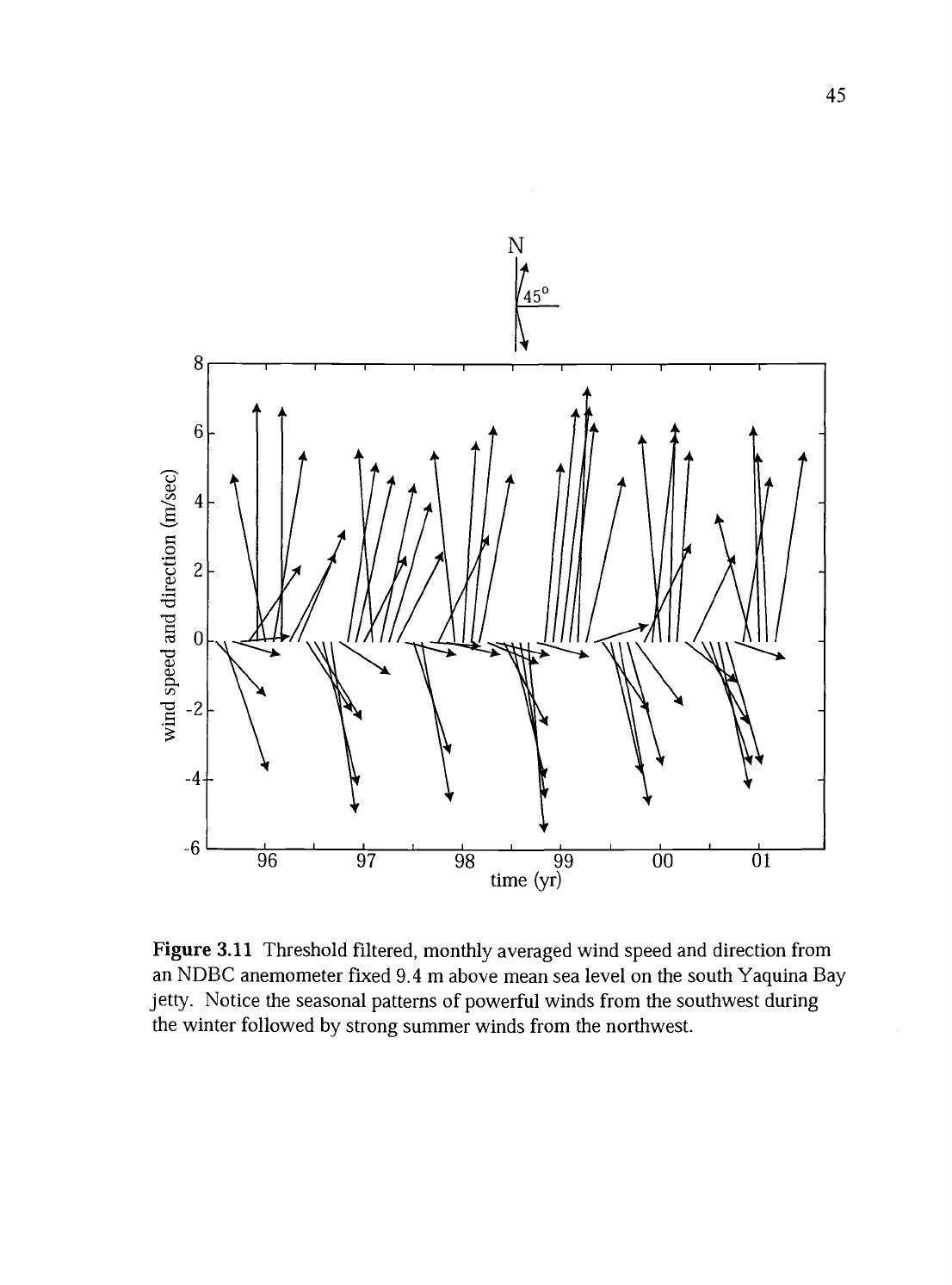
Figure 3.11 Threshold filtered, monthly averaged wind speed and direction from
an NDBC anemometer fixed 9.4 m above mean sea level on the south Yaquina Bay
jetty. Notice the seasonal patterns of powerful winds from the southwest during
the winter followed by strong summer winds from the northwest.

to the survey points by minimizing mean square deviations between the model and
survey data. Besides providing elevation estimates at the grid nodes, the Loess
filter interpolation technique supplies smoothing for variability at scales shorter
than a user determined cutoff. This cutoff determines the wavelength of features
that can be resolved in the interpolated field. Isotropic correlation length scales of
100 m were applied in order to limit the occurrence of missing interpolation
estimates within the time series resulting from sparse sampling. This smoothing
allows resolution of features with wavelengths 200 m or more in the cross-shore
and alongshore directions (Figure 3.1 2a). Areas of the beach with short scale
variability (e.g. the seasonal dune field discussed earlier) are effectively smoothed
over. Most important, the Loess technique provides error estimates due to
interpolation uncertainty (Figure 3.12b). High errors in the interpolation field can
result from large spatial gaps between survey observations. However, in the
interior of the sampling region the typical interpolation uncertainty produced by the
Loess technique at the previously mentioned smoothing scales is O(0.005m).
Similar to Plant and Holman (in review), grid nodes with interpolation errors above
0.lm have been removed from each gridded survey set.
The alongshore curvature of Agate Beach produces inconsistencies in the
directions for cross-shore and alongshore estimations of sediment flux within the
current local coordinate system (Figures 2.2). It is necessary to remove this
curvature in order to get at the local cross-shore and along shore orientations of the
beach. First, a circle is regressed on to the time averaged horizontal position of the

47
a
5
b
0.1
10001
':,
1000
Li
0.09
1
4
0.08
500
f /
sooj1
J
3
H
0.07
1
'
0.06
-'
-S
0
0.
c'
2'
I, C
o
0
'1fllZ
'.J.'J.)
Q_)
-
I
>
0.04
-500
1
-500
0.03
(I.
I
0
i ()()()
1000
0.02
-1
0.01
-1500
-1500
0
0 200 400 600
0 200 400 600
cross-shore (m)
cross-shore (m)
Figure 3.12 RTK-GPS gridded data and interpolation errors from a topographic
survey of Agate Beach on November 11, 2000 a) The gridded beach surface
with
nodes separated by 10 m in the cross-shore and 20 m in the alongshore. The colors
represent elevation, and contours are shown in 1 m intervals. b) The error calculation
at each grid node due to interpolation uncertainty. Note the extremely low error in
the center of the survey region.

im elevation contour (Figure 3.13). The radius of the circle fit (ro) is extended to
contain the survey region within the circle boundary
(rext)
(Figure 3.1 4a). Next, the
local coordinate system origin is translated to the center of the circle. We then
define a domain
D
as the region bounded by the circle and transform the local
coordinate system into complex space Z.
Z=x +iy
(13)
The transformation of the domain
D in complex Z space, to a domain
D*
in
complex space W, where the cross-shore position of elevation contours remains
constant, is done using a linear fractional transformation (O'Neil, 1995, Figure
3.14b).
1. Normalization to the unit disk
=
Z
(14a)
ext
2. Fractional Transformation
W' = T(Z')
(Z' +1)
(1 4b)
(z' 1)
3. Magnification and Translation
w
= r,
W' +
iy0
(1 4c)
yo = alongshore center of the circle in the original local coordinate system
The black cross-hatched lines in Figure 3.14a are separated by 50 m in the cross-
shore and alongshore directions. Figure 3.14b shows the minimal distortion of
those regularly spaced grid lines resulting from mapping Z space to W space. The
domain of interest,
D*,
is a small area with respect to the total area of the circle and

1000
500
0
C,.)
0
-500
-1000
-1500
cross-shore (m)
- - circle fit
im elevation
I
5
contour
4
3
2o
>
[I]
-1
-2
Figure 3.13 The time averaged gridded beach surface over the 27 survey
topographic record.

Z Space
W Space
(a)
1000
(b)
1000. -
- Il
rrum L
50C
I-
C
C,,
C
50(
-1 O0(
-150
5
500
3
0
C
>
-500
0
-1000
-1
-2
-1500
cross-shore (m)
cross-shore (m)
5
4
3
2
1
-1
-2
C
a.)
a)
50
Figure 3.14 The transformation of the mean beach surface from Z to W space. a)
The mean beach surface with elevation contours and the circle boundary of the beach
region dashed in red. Note the alongshore curvature of the elevation contours in Z
space. b) The mapping of the mean beach surface into W space,
where the elevation
contours and circle boundary become lines. Cross-hatched lines in (a) are spaced
50m in the cross-shore and alongshore. The same pattern is mapped into W space to
show the minimal amount of horizontal distortion caused by the mapping.

51
is also located very near the circle boundary. Because of these two factors, the
maximum horizontal distortion, 0(0.1 m), caused by the linear fractional
transformation occurs near the alongshore extremes of the domain, D*. Here, we
define distortion as the change in unit length in the x andy directions caused by the
transformation.
3.4.2 Beach Surface Change Analysis
After the alongshore curvature of the beach has been removed, the patterns
of local cross-shore and alongshore sediment flux are more readily identifiable.
Figure 3.15 shows mean, standard deviation, and skewness maps of the gridded
beach surface over the complete survey time series. Grid nodes with less than 50%
of the total number of observations have been removed from all of the remaining
analysis (Figure 3.16). The channel morphology related to Big Creek and Little
Creek near y = 0 m andy = -500 m are well-resolved features in the time averaged
beach surface. Besides these two areas influenced by the creeks, the mean beach
surface shows little alongshore structure. The standard deviation map in Figure
3.1 5b illustrates the spatial structure of the beach surface variability over the 6 year
record length. It is important to note that the beach response is not cross-shore
uniform. Instead, Agate Beach exhibits increased amounts of surface variability
located in the backshore near Big Creek and in 2 alongshore parallel bands around
x = 200 m and 400 m. The patch of high variability associated with Big Creek
(O>y>-600 m) is due to the migration of the creek channel to the north (observed in

0
0
0
(a)
1000
500
-500
-1000
14
(b)
1000
500
12
C
N
1
-500
Jo
I-i
-1000
(c)
1000
10.6
500
0.5
0
0.4
0.3
-500
0.2
-1000
10.1
2
1.5
0.5
0
-0.5
-1.5
-1500
-
-1500
-
-1500 -2
0
500
0
500
0 500
cross-shore (m)
Figure 3.15 Statistics of surface variability at Agate Beach over the survey record
length. The alongshore curvature of the beach has been removed, a) The time
averaged beach elevation surface,
b) The standard deviation map with respect
to z, o, illustrates the alongshore and cross-shore structure of surface changes. c)
The skewness map, y, is dominated by positive values, indicating that most of the
observations throughout the record occur below the mean beach surface elevation.

1000
500
0
0
-500
-1000
I,
500
cross-shore (m)
26
24
22
20
z
18
16
14
12
10
''1
Figure 3.16 The number of observations (N) at each grid node over the 27 survey
record length.

54
the Argus video record in 1996) as well as channel cutting and fill from large
seasonal changes in rainfall and discharge. The alongshore bands of increased
variability are good indicators as to the cross-shore behavior of the beach response.
In the cross-shore direction, there are distinct locations with a greater sediment
response to changes in wind and wave forcing that will be discussed later. The
skewness map (Figure 3.15 c) indicates that the majority of the observations at each
grid cell are positively skewed. Therefore, the majority of the beach is more often
observed below the time averaged beach surface elevation. This is a result of the
irregular sampling interval shown in Figure 2.4. Because 16 of the 27 topographic
surveys are found in the 1995-96 survey series, skewness statistics are biased
toward a beach containing less sediment. The range map shown in Figure 3.17, is
calculated by subtracting the minimum elevation value from the maximum value at
each grid point in the survey record. By summing over the range map a volume
difference of
l.30x106 m3
quantifies the dynamic volume of sediment involved in
transport processes along the beach over the survey record length.
Removing the alongshore curvature of the beach also allows us to make
alongshore averaged calculations of the mean beach profile, standard deviation, and
skewness as a function of cross-shore position (Figure 3.18). The alongshore and
time-averaged profile illustrates the shallowing of the beach slope with increasing
offshore distance that is typical of beaches exposed to high incident wave energies.
A plot of the alongshore-averaged standard deviation, o, shows two dominant
bands of beach elevation variability in the cross-shore direction (Figure 3.18b).

1000
500
S
2.5
IL2
500L31)j
j'
1000
Li
05
l500o
200
400
cross-shore (m)
Figure 3.17 The range in elevation at each grid node calculated by subtracting the
minimum elevation from the maximum elevation observed throughout the survey
time series. Note some regions of change up to 3m in elevation.

0
>
C.)
C.) -,
0.
C
0.
0.
C
C
(a)
envelope
0
100
150 200 250
300 350
400
450 5
iOU
150
200
250
300
350
400
450 51
1
0.5
'-'< 0
-0.5
\Y
15Q
iOo i
4000
3000
05
1601
cross-shore (m)
(c)
56
Figure 3.18 The alongshore averaged statistics of the Agate Beach survey time
series, a) The mean beach surface elevation profile. b) The standard deviation
profile reveals a decrease in surface variability around x = 300 m, surrounded
by two distinct bands of higher variability. c) The skewness profile shows a
switch from negative to positive values at x= 150 m. The beach seaward of
that point is more often observed below the mean surface elevation, while areas
landward are more often found above the mean elevation profile. d) The
number of observations at each cross-shore location.

57
The band from 1 50<x<275m will be shown later to correspond to the wind-driven,
seasonal dune field that develops during summer months. The second band of
increased variability occurs seaward of x = 300 m. This area is continually under
the influence of swash and hydrodynamic sediment transport processes directly
related to the offshore wave climate.
The alongshore averaged skewness profile,
'yr,
(Figure 3.1 8c) reveals some
cross-shore structure with a node at x = 150 m. Seaward of x = 150 m the skewness
remains positive, indicating that the majority of observations found at cross-shore
positions greater than x = 150 m lie below the mean elevation for that position. On
the contrary, all grid nodes landward of x = 150 m are negatively skewed.
Therefore, around x = 150 m there is a node where the beach surface responds
differently on both the landward and seaward sides. It is also worth noting that this
result may be a product of the bias created by inequality in sampling between the
two survey series (Figure 2.4).
Perhaps a more interesting way to analyze the variability in the survey data
is by examining the variation of statistics with vertical elevation. Gridded elevation
values throughout the survey record are binned in 5 cm increments from z = -2.525
m to z = 5.025 m. The time averaged cross-shore position and range of each
elevation bin are plotted in Figure 3.1 9a showing the gently sloping nature of the
mean beach surface. The standard deviation profile with respect to elevation, o,
(Figure 3.1 9b) reveals a decrease in variability near the 1 m elevation contour.
This dip in the profile indicates an elevation contour in the beach surface that

a
0
200
C
400
C)
N
-
d
2000
1500
Z 1000
500
0
I
I
I
I
5 4 3 2 1 1) -1 -2 -3
elevation (m)
58
Figure 3.19 Statistics of Agate Beach as a function of surface elevation, a) The
time-averaged cross-shore position and range of each 5
cm elevation bin. b) The
standard deviation for each elevation bin reveals a decrease in cross-shore
variability near the 1 m elevation contour. c) Similarly, the skewness profile
resolves a node near the 1 m elevation contour. Elevations above 1 m are
negatively skewed while elevations below 1 m are positively skewed. d) The
number of observations in each elevation bin.

responds less to forcing than both higher and lower elevations. Furthermore, the
skewness map with respect to elevation, y, (Figure 3.1 9c) reveals a node around
the same 1 m elevation contour. Elevations higher than the 1 m contour are more
regularly observed seaward of their mean position due to negative skewness, while
elevations lower than 1 m are more often observed landward of their mean position
as a result of positively skewed values. Again, these results may also be a product
of sampling bias shown in Figure 2.4.
Analysis of the survey data with respect to elevation shows that the beach
surface responds in distinct bands of variability on either side of the 1 m elevation
contour. Interestingly, the NOAA tidal gauge in Yaquina Bay estimates mean high
water (MHW) at z = 1.076 m and mean higher high water (MHHW) at z = 1.283 m.
The bands of increased variability around the 1 m elevation contour suggest an
interesting separation in the beach profile response. The cross-shore profile
behaves as the combination of a wave driven response that tapers away above
MHW, and an aeolian dune response that is limited to the region above MHW.
An empirical orthogonal function (EOF) analysis of the survey record
identifies the spatial and temporal patterns of beach surface variability (Winant et
al., 1975, Davis, 1976). Due to large changes in beach surface elevations between
the 1995-96 and 2000-0 1 survey series, the elevations from each survey are
normalized to unit range in order to better resolve the intra-annual patterns of
surface variability.

The EOF decomposition of the survey record produces two distinct modes
explaining 34% and 21% of the normalized variability (Figure 3.20). In our
previous analysis of the topographic surface data we have shown where the beach
responds to changes in forcing. The EOF analysis not only decomposes the
variance into independent spatial patterns of variability, but also provides a time
signature related to these modes of variance.
The spatial pattern of the first mode is relatively alongshore uniform
suggesting a response due to cross-shore fluxes of sediment. The alongshore mean
of the spatial pattern outlines a cross-shore profile that is dominated by a backshore
beach response (Figure 3.20a). This mode describes the dune field that emerges in
the backshore next to the seacliff during the drier summer months. The temporal
pattern of the first mode is correlated to an armual amplitude signal that is more
readily visualized in Figure 3.21. In the top panel the first year survey time series
(1995-96) of the EOF mode 1 amplitude signal is shown. During the summer and
early fall months, the amplitude of the first mode increases, making the growth of
the dune field in the backshore an important part of the beach surface variability.
Along with the (1995-96) amplitude time series of the first mode, a periodic, annual
(10
=2m/365 days') signal is plotted to show the seasonal nature of the dune mode.
In the lower panel (Figure 3.21 b), the corresponding monthly statistic for
wind speed and direction are plotted for a comparison with the dune mode
amplitude time series. When the wind is strong and from a southerly direction, the
amplitude of the dune mode decreases. Figure 3.22 plots the monthly mean

0
0
61
0.08
0.06
0.04
0.02
0
-0.02
-0.04
0
500
cross-shore (m)
0.08
1000
0.06
500
0.04
0
bo
0
0
-500
-0.02
0.'
0.1
0.05
l000I_.1
-0.04
0
-0.05
n
/
time (yr)
EOF Model
100 200 300
400
500
cross-shore (m)
EOFMode2
L
7
8 99
do
di
time (yr)
100
200
300
400
500
cross-shore (m)
cross-shore (m)
Figure 3.20 EOF analysis of the normalized survey, record reveals two distinct
modes of surface variability. The first mode (34% of the variance) suggests a
pattern related to the seasonal backshore dune field that forms during the summer
months. An alongshore average of the mode shows the cross-shore structure of the
dune pattern. The amplitude time series of the first mode reveals a seasonal cycle
related to dune growth in summer and loss of sediment in this region during winter.
The second mode (21% of the variance) appears to be related to the seasonal
changes in the rest of the beach surface elevations outside of the dune area.

2.5
00.5
0
0
-u
(/)
-u
.-,.
U
_I) .
62
I
I I
I
I I I
I I
(a)
1995
1996
I
I
I
I
I
I
I
jun jul
aug sep
oct nov dec
jan
feb
mar apr may jun
jul
(b)
]un jul
aug sep
oct nov dec
jan
feb
mar apr may jun jul
Figure 3.21 The dune mode EOF and monthly wind time series, a) The first
year of the amplitude time series from the dune mode EOF (1995-96). A
periodic, annual signal is plotted with the EOF time series to show the seasonal
behavior of the dune mode. b) The monthly averaged wind speed and direction.
Note the correlation between the seasonal dune mode amplitude and the wind
time series. The erosion and disappearance of the dunes corresponds with the
onset of the strong, southerly winds associated with winter.

2
1.5
1
0
0.5
I
63
2
0 -2 -4 -6
-8
-10
l/WJfld(m/sec)
Figure 3.22 The monthly mean alongshore wind velocity vwjnd plotted against
the dune mode EOF amplitudes from the 1995-96 survey record showing the
correlation between strong northwest summer winds and the growth of the
backshore dune field.

alongshore wind velocity
(v,I,Ed)
verses dune mode amplitudes from the 1995-96
survey year. The correlation between
V,Ed
and the dune mode amplitudes (p = 0.45
with
Pcrit
= 0.36 at 95% confidence level) relates the emergence of the backshore
dune field to the northwest winds characteristic of the summer months. Probably
more important in the building of the dune field is the lack of swash interaction on
the upper beach. Without strong southern winds, setup is decreased as well as the
lack of extreme runup from the larger waves characteristic of winter conditions. At
the same time, precipitation levels fall dramatically. This allows the upper beach
sediments to sufficiently dry and enables aeolian transport to dominate the
sediment fluxes along the seacliff without the erosive nature of high energy swash
and rain saturated conditions.
The second EOF mode describes a pattern related to the variance associated
with the rest of the beach. This mode also shows little alongshore structure. The
alongshore mean of the spatial pattern reveals a cross-shore profile response
corresponding to the beach surface seaward of the region dominated by the dune
mode (Figure 3.20b). Similar to the first mode, the amplitude time series of this
beach mode reveals an annual pattern. During the summer and early fall of the first
year of the amplitude time series, the positive values of the spatial pattern
contribute to the beach variance. This is followed by winter months, where the
amplitude time series switches sign and therefore the spatial pattern of the second
mode becomes largely negative, stripping sediments from the beach. The
alongshore uniform structure of both of the modes produced by the EOF analysis

suggest cross-shore sediment fluxes dominate the patterns of variability along
Agate Beach on a seasonal cycle.
Estimates of net alongshore and cross-shore sediment fluxes,
Q,,
can be
made based on calculation of time variations of the total sediment volume in the
survey region. The volume contained within the box (Figure 3.23) is calculated as:
Vb(t)=z(t,x,yJ)\xz\y
(15)
where Ax = 10 m, Ay = 20 m and only grid nodes that contain no missing data are
used. The mean volume is then removed to produce the
Vb(t)
time series shown in
Figure 3.24. The
Vb(t)
time series is modeled after equation 2 using a least squares
multiple linear regression. The fit to the data,
Vmodel,
is significant at the 95%
confidence level with R = 0.97 and
0.14.
The alongshore uniform structure of the EOF spatial patterns and periodic
nature of their temporal signatures suggest they are strongly related to a nearly
balanced seasonal cross-shore
flux
of sediment (Figure 3.20). Assuming the net
cross-shore flux
(Q)
within a year is close to zero, we model the change in beach
volume
Vb(t)
as a periodic, annual cross-shore sediment
flux (Q)
superimposed
upon an interannual alongshore sediment
flux (Q)
to the north.
Q is
decomposed
into a periodic signal described by a cyclical component and çbv = -0.27 yf' with a
net annual transport of zero. Furthermore, assuming that Yaquina Head acts as a
barrier to alongshore sediment transport, forcing alongshore transport gradients to
zero at the headland, the
fl
term in equation 2 corresponds to the net rate of
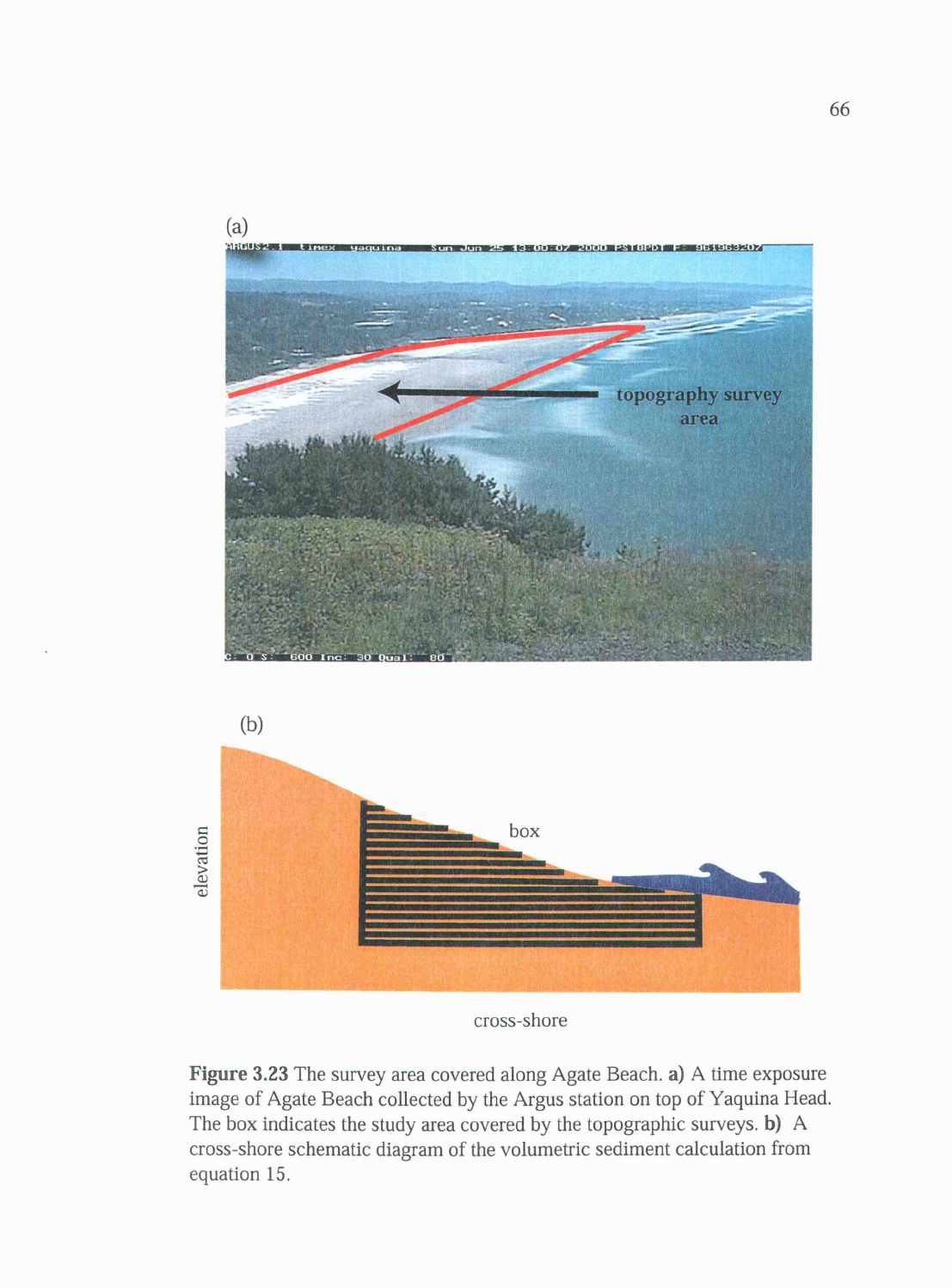
USZ.1
tne
yeg,.n
S,n Jr 25 l3OO:O7 2UUO PST8POT F
961IJO7
area
(b)
0
Ct
cross-shore
Figure 3.23 The survey area covered along Agate Beach. a) A time exposure
image of Agate Beach collected by the Argus station on top of Yaquina Head.
The box indicates the study area covered by the topographic surveys. b) A
cross-shore schematic diagram of the volumetric sediment calculation from
equation 15.

2.
-2
67
J
I
I I
I
I I
I I I
*
*
I,
1
I'
1
I
I
S
,
t
I
I
)
I
I
I
I
I
'
I
t
I
I
I
I
5 I
'
1
ft
I
'I
*%4*
RTK-GPS
I
*
.lidar
--model
I
I I I
I I I
I I
I
95
96
97
9A
99 00
01
time (yr)
Figure 3.24 The demeaned beach volume time series, V calculated from all of
the topographic surveys. The dashed line represents a multiple least squares
regression fit to beach volume estimates. The regression model is composed of a
periodic seasonal cycle, an increasing linear trend, and an offset.

northward alongshore sediment transport Q)' = 3.325x10⁴rn3/yr. This is a net rate
calculated over the survey record and a result of the accumulation of sand within
the study area. A more exact description of
would be defined from more
frequent topographic sampling around episodic storm events that could be
compared to estimates of Qi from the wave conditions presented in section 3.2. A
comparison between estimates of Q, and Q' is discussed in chapter 4.
3.5 Video Data Analysis
Spatial measurements from video images are made by transforming
intensity values from pixel space (U and 17) to the right hand local coordinate
system common to the topographic survey data (x andy). The transformation from
pixel space to real world coordinates is accomplished by standard photogrammetric
techniques involving the geometric description of the camera position relative to
the known positions of objects within the images (Holland et al., 1997). Each pixel
in an oblique image (Figure 2.8) has an infinite number of corresponding real-
world coordinates. However, by choosing the vertical coordinate to correspond to
mean sea level, a unique map view, or rectification, can be computed (Figure
3 .25a).
Three cross-shore transects are chosen from the straightened beach in W
space (section 3.4.1). These coordinates (x' andy) are transformed into the local

(a)
1000
800
600
400
200
-200
-400
-600
-800
-1000
-1200
0
(b)
400
800
cross-shore (m)
1200
I I
I I
I
= 0
-
-
..y=-500
'4 , '4
y=-1000
I
/ - - -
3.)
.. -...
ThTTT'ThT
0 100
200
300
400 500
600
700
800
900
1000
cross-shore (m)
Figure 3.25 a) A rectified or plan view of the "daytimex" image from Figure 2.7 in
local coordinates. Note the cross-shore transects have been corrected for the
alongshore curvature of the beach. b) The pixel intensity profile corresponding to
each of the cross-shore transects shown in (a). The peaks in intensity correspond to
the cross-shore position of the sand bars.

70
coordinate system (x andy) by the inverse of the complex mapping described
earlier (W space to Z space). From each daytimex image, intensity values
corresponding to pixels nearest the x andy coordinates of each transect are
interpolated onto those positions. This provides intensity estimates spaced at 5 m
cross-shore intervals for 3 alongshore locations (Figure 3.25b).
Cross-shore intensity profiles from each daytimex image are used to build a
space-time slice of image variability (I(x, t)) known as a timestack (Figure 3.26,
Aargard and Hoim, 1989, Holland and Holman,1993). Time stack images resolve
the time varying cross-shore position of the sandbars and shoreline. The timestacks
are low-pass filtered in space to remove higher wavenumber variability using a
Hanning window with a filter cutoff
K<
0.0125 m4. Since the intensity range
across each transect varies due to changes in insolation (e.g. cloud cover, seasons),
each cross-shore profile is normalized to unit range.
Some bias may be introduced into our analysis due to the fact that wave
breaking must occur over the sand bars in order for this optical method to resolve
the cross-shore position of bathymetric highs. Thus measurement of the cross-shore
position of the furthest offshore sand bars may be overly sensitive to surf zone
width. However, because Agate Beach is continuously exposed to high wave
energy, our technique appears to perform well with respect to locating the general
cross-shore position of the outer sand bar.
The filtered and normalized timestacks provide a basis to analyze long-term
sand bar behavior at Agate Beach. A measure of the time varying cross-shore

y=Om
1993
1994
1995
1996
1997
1998
1999
2000
y=-500m
1993
1994
1995
1996
1997
1998
1999
'S.'
y=-l000m
71
2001 2001:
2001
200
600 1000
200 600
1000
200
600
1000
cross-shore (m)
Figure 3.26 The normalized timestacks composed of "daytimex" images from the 3
cross-shore profiles shown in Figure 3.25. Note the periodic, seasonal nature of the
bright bands of intensity related to the position of the offshore sand bars. Also
important are the bright bands of intensity occurrIng in the backshore during the
summer months. These areas are associated with the bright reflection of sunlight off
the dry sand in the summer dune field.

72
position for the most seaward sandbar (ob) at each alongshore location is made
with a second order Canny edge detection algorithm smoothing over one week
intervals (Figure 3.27, Holland and Holman, 1996). An alongshore average of
results from the three transects is used to estimate the time history of the general
cross-shore location of the outer sandbar,
OB,
over the -9 year video record
(Figure 3.28).
To characterize the time varying cross-shore behavior of the outer bar, the
OB
time series is modeled after equation 2 using a multiple linear least squares
regression. The model fit, OBxmod, is significant at the 95% confidence level with
R2
= 0.68 and R2crit = 0.54 using Chelton's (1983) estimate for N* = 14. OBxmod is
comprised of periodic intra-annual variability (w = 2it/365 days'), an inter-annual
long-term offshore trend and an offset. The periodic seasonal cycle has an
amplitude
AOB
= 114.86 m and phase
q5OB
= 0.28
yf' describing the offshore
migration of the outer sand bar during winter and onshore return during summer
conditions similar to the behavior of Vmodel from section 3.4.2. The long term,
inter-annual seaward trend
(foB = 11.0
m/yr) in the cross-shore position of the
outer sand bar described by OBxmod also shows agreement with the long-term
increase in beach volume described by Vmodel. Long-term growth in the volume of
beach sands along Agate Beach corresponds with a seaward trend in the periodic
annual migration of the outer sand bar.

73
01/01/93
01/01/94
0 1/0 1/95
0 1/0 1/96
01/01/97
0 1/0 1/98
01/01/99
01/01/00
01/01/01
y=0m
100 200 300
400 500 600
700 800 900 1000
cross-shore (m)
Figure 3.27 The "daytimex timestack history of the cross-shore intensity
profile at y = 0 m. The cross-shore position of the seaward edge of the outer
sandbar (ob, is acquired from a second order Canny edge detection
algorithm.

74
01/01/93
01/01/94
0 1/0 1/95
01/01/96
01/01/97
0 1/0 1/98
0 1/0 1/99
0 1/0 1/00
01/01/01j
400
500
_____- -
600
JUU
cross-shore (m)
Figure 3.28 The alongshore averaged, cross-shore position of the outer sand
bar, OB. The dashed line represents the least squares multiple linear
regression fit to the OB time series after equation 2. The regression model,
OBxmod is composed of a periodic, annual signal superimposed on a longer
term offshore trend. This is consistent with the overall increase of sediment at
Agate Beach described in section 3.4.

75
Chapter 4 DISCUSSION
The time series' of statistics describing the wave climate forcing and
sediment response modeled in the previous sections are summarized in Table 4.
The seasonal periodicity in both the forcing and sediment response are
characterized as variance about a long-term, linear trend better defined as Large
Scale Coastal Behavior,
LSCB.
The long- term increasing trend in H (/J= 6.7
cm!yr) coupled with the low frequency reorientation in 9
(fio=
southlyr) combine
to drive an aecretionary regime at the northern end of the Newport littoral cell.
Similarly, the
LSCB
observed in the /3v and
/3OBx
terms describing the long-term
growth in sediment volume of the subaerial beach and the offshore migration of the
outer sand bar support our hypothesis of net northward sediment transport and
accumulation along Agate Beach. These results are also consistent with the
expected sediment transport patterns associated with the 1997-98 El Niflo and
1998-99 La Nina sequence. Except for
Vb,
an order of magnitude difference
between the seasonal component of the modeled variability, A, and the long-term
component, f3, suggests seasonal variance dominates the signals on an annual
basis.
The timing of the seasonal beach response to wave forcing is well resolved
within the phase information obtained from the models. From Table 4 a yearly
cycle generally proceeds as follows. In October
I-Is and T begin to increase,
followed by a shift to a more southerly approach in 0. Similarly, the offshore

76
Table 4 Comparison of model coefficients for wave climate, beach sediment
volume, and outer sand bar position. Confidence intervals are evaluated at the 95%
level.
Parameter
(yf')
13x0
H3
0.94 m
± 0.06
0.36 ±
0.04
6.7 cm/yr ±
2.42 m ± 0.03
2.6
T
2.lsec±O.1
0.35±0.05
0.l5sec/yr± 11.Osec±
0.04
0.06
9
12.3°±2.0
0.30±0.10 3° S/yr±0.8
-3.5°± 1.0
Vb
7.85x10⁴ m3 ±
-0.27 ± 0.12
3.33x10⁴
-8.46x10⁴ m3 ±
2.13x10⁴ m3/yr±
1.52x10⁴
4.6x10³
OB
114.9 rn
± 4.2
0.28 ± 0.04 11.0 rn/yr ± 635.7 m ± 4.2
0.8
migration of
OBxmod
lags the increase in
H3 by roughly a month. Lastly, the
decrease in the volume of sand on the beach lags the increase in H3 by 45 days.
Then, during spring conditions
I-Is
begins to decrease, followed by the return of
OBxmod,
and lastly, an increase in the volume of sand on the subaerial beach. This
study quantifies the phase lag in the sediment response to the wave forcing. This is
a crucial point in arguments between equilibrium and dynamic theories for cross-
shore beach profile models. The observed phase lag of roughly 45 days between H3

77
and
Vb
lies midway between the zero phase lag expected for equilibrium profile
models and phase lag of rt/2 expected for dynamic models.
Evaluating the performance of the predicted values of net alongshore
transport from wave climate information (
Wnet
=
2.73x10⁸ m3
north) with the
measured values from topographic analysis
(AVby
1 .84x105
m3) reveals good
agreement in the direction of transport to the north. However, the predicted
magnitude of the transport is roughly 1500 times greater than our estimates from
topographic data. The net increase in volume due to alongshore transport,
AT7by, is
calculated by subtracting the volume of the beach surface from the
Vb
time series
when at its maximum in September 1995 from the maximum in September 2000.
Since we attribute the long-term trend in the
Vb
time series to alongshore sediment
flux, the net gain between maxima reveals the alongshore contribution of sediment
to the study area.
The disagreement between the predicted and measured values of sediment
transport may be related to the fact that Agate Beach is not a perfectly closed
system. Leakage of sediment to the north around the headland during extreme
wave events is likely. Our value for the predicted alongshore transport also
neglects any aeolian influence during the sumn-ier season, which as we have shown
is an important component of both the cross-shore and alongshore flux of sediment
at Agate Beach. By including wind transport of sediment during the summer
season, which would tend to remove sand to the south away from our study area,

78
better agreement in the predicted and measured alongshore sediment flux may be
reached.
Discrepancies in our estimates of Qi from offshore buoy statistics versus
those used by Komar (1970) at the breaker zone may also contribute to slight errors
in net transport calculations. Wave momentum flux (S) must be conserved from
deep water to the break point. Combining equations 7 and 8 yields
I1=KcS,
(16)
where both K and S remain constant. The ratio between estimates of alongshore
sediment flux from deep water wave measurements (Qideep) and Komar's (1970)
estimates at the break point (Qlbp) can then be revealed using equation 9.
Qideep
'Ideep
C
deep
Qmp
'lbp
Cbp
(17)
From linear Airy wave theory
g7eep/
Cbp
.,jghb
(18)
where Tdeep is the deep water wave period and hb represents the depth of breaking.
Using values of Tdeep = 10 seconds and hb = 4 m typical of Agate Beach, the ratio
between deep water and break point estimates of alongshore sediment flux
(Qldeep/Qmp) is rougly 2.5. This value is far less than the O(10) discrepancy
observed in the measured and predicted sediment flux values.

79
Another source of error in the comparison between predicted and measured
alongshore sediment flux may be due to a limited survey region. The long-term
offshore migration of OB suggests sediment accretion over a much wider cross-
shore region than the measured topographic survey area. Although, a portion of the
long-term signal in OB may also be the result of the overall increase in H forcing
the break point further offshore.
Analysis of the topographic survey data reveals the cross-shore structure of
the time varying response of the beach surface to changes in wave and wind
forcing. Alongshore parallel bands of increased variability around the im elevation
contour coincide with distinct processes. The landward band is related to a
seasonally wind generated dune mode that evolves during summer and early fall
and is limited to the region above MHW. The seaward band of high variability is
associated with a wave-driven mode affecting the remainder of the beach surface
below MHW.
The analyses of wave forcing as a driving mechanism for
LSCB along
Agate Beach is dependent on scale. The focus of this analysis is on larger scale
changes spanning several years. By smoothing beach and sandbar variability at the
appropriate temporal and spatial scales, good evidence exists for the directly forced
beach response. At finer scales instabilities in the beach configuration may become
important as feedback mechanisms for the overall beach evolution. For example,
smaller scale rip channels and complex bar morphologies may contribute to the
overall sediment transport offshore and alongshore by influencing the flow. These

types of smaller scale features contribute to the alongshore structure of the beach.
In aggregate these features may bring the beach to a similar state as that predicted
by the direct forcing from larger scale changes in wave climate. Still, for this study
the long-term and seasonal behavior of the beach system at larger spatial scales
appears to be directly forced by annual and lower frequency variability in the wave
climate.
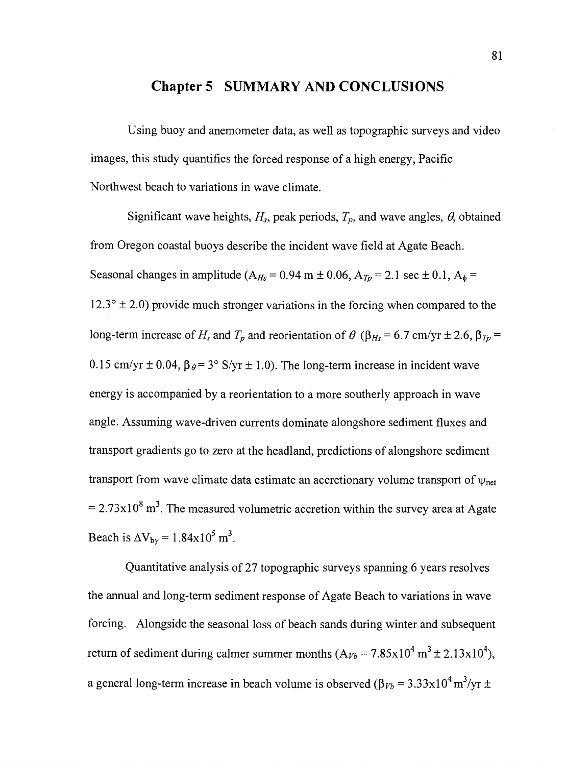
81
Chapter 5 SUMMARY AND CONCLUSIONS
Using buoy and anemometer data, as well as topographic surveys and video
images, this study quantifies the forced response of a high energy, Pacific
Northwest beach to variations in wave climate.
Significant wave heights,
115, peak periods, Ti,, and wave angles, 9, obtained
from Oregon coastal buoys describe the incident wave field at Agate Beach.
Seasonal changes in amplitude
(AHS = 0.94 m ± 0.06,
AT
2.1 sec ± 0.1, A =
12.3° ± 2.0) provide much stronger variations in the forcing when compared to the
long-term increase of
H5
and T and reorientation of 9
(13Hz
= 6.7 cm/yr ± 2.6,
I3Tp =
0.15 cm/yr ± 0.04, 138 = 3° S/yr ± 1.0). The long-term increase in incident wave
energy is accompanied by a reorientation to a more southerly approach in wave
angle. Assuming wave-driven currents dominate alongshore sediment fluxes and
transport gradients go to zero at the headland, predictions of alongshore sediment
transport from wave climate data estimate an accretionary volume transport of
Wnet
= 2.73x10⁸
m3. The measured volumetric accretion within the survey area at Agate
Beach is AVby =
1.84x10⁵ m3.
Quantitative analysis of 27 topographic surveys spanning 6 years resolves
the annual and long-term sediment response of Agate Beach to variations in wave
forcing.
Alongside the seasonal loss of beach sands during winter and subsequent
return of sediment during calmer summer months (Avb = 7.85x1 0 m3 ± 2.1 3x1 0),
a general long-term increase in beach volume is observed (I3vb = 3.33x10⁴ m3/yr ±

4.6x10³). Unlike the
wave climate variables, the magnitudes of seasonal and long-
term sediment volume changes are very similar. Elevation change estimates over
the record length are large with some regions of the beach exhibiting elevation
gains up to 3 m. Consistent with the long-term growth in subaerial beach volume,
-9 years of video data show a steady long-term offshore migration rate of the outer
sand bar
(13
OBX
= 11.0 rn/yr ± 0.8). This long-term offshore migration is coupled
with seasonal fluctuations in cross-shore position
(A0BX
= 114.9 m ± 4.2) as a
response to variations in wave climate.
Besides describing the response of the beach in terms of sediment volume
and cross-shore position of the outer bar, this analysis also decomposes the cross-
shore structure of the time varying beach surface using 2 eigen modes. The first
mode is characterized by the seasonal growth of a dune field explaining 34% of the
variance in the data. This mode of variability is limited to elevations above MHW.
The dune mode is wind forced and correlated to summer winds and lack of
precipitation and swash above MHW. The second mode describes the seasonal
variability in the beach surface related to wave driven processes. This mode
explains 21% of the variance and describes the beach surface changes below the
MHW. The cross-over between these modes of variance is observed around
MHW elevation at z = 1.076 m. Landward and seaward of MHW, the beach
responds to forcing in two alongshore bands of increased variability.
Although the regression models developed in this analysis quantitatively
describe the seasonal and long-term variability in both the forcing and response of

83
the Agate Beach system, an improved description of the LSCB can be obtained by
continued topographic surveys and collection of video, buoy and anemometer data.
The long-term increasing trends identified in this analysis may actually represent
portions of lower frequency variability that is not resolved within the current record
length. Perhaps these trends in wave climate forcing are related to long-term
oscillations in regional oceanic conditions as suggested by Allan and Komar
(2000).

REFERENCES
Aagard, T., and J. Hoim, 1989, Digitization of Wave Runup Using Video Records.
J. Coastal Res., 5,547-551.
Allan, J. and P.D. Komar, 2000, Are ocean wave heights increasing in the eastern
north pacific? EOS Trans., Amer. Geophys. Union, 8 1(47), 56 1-567.
Aubrey, D.G., 1979, Seasonal patterns of onshore! offshore sediment movement. I
Geophys. Res., 84, 6347-6354.
Aubrey, D.G., 1983, Beach changes on coasts with different wave climates. Sandy
Beaches as Ecosystems: Dr. W. Junk Publishers, The Hague, 63-86.
Bagnold, R.A., 1984, The Physics
of
Blown Sand and Desert Dunes. Chapman and
Hall, London New York, 256
pp.
Birkemeir, W.A., 1984, Time scales of nearshore profile changes. Proceedings
Coastal Engineering '84, New York, ASCE, 1507-1521.
Birkemeier, W.A., H.C. Miller, S.D. Wilhelm, A.E. DeWall, and C.S. Gorbics,
1985, A User's Guide to CERC's Field Research Facility. Coastal Engineering
Research Center, U.S. Dept. of the Army, Waterways Experiment Station, Corps of
Engineers, Instruction Report CERC-85-1.
Bowen, A.J., 1969, The generation of longshore currents on a plane beach. .1.
Marine Res., 27, 206-215.
Chelton, D.B., 1983, Effects of sampling errors in statistical estimation. Deep-Sea
Res., 30, 1083-1103.
Dail, H.J., M.A. Merrifield and M. Bevis, 2000, Steep beach morphology changes
due to energetic wave forcing. Mar. Geol., 162, 443-458.
Davis, R.E., 1976, Predictability of sea surface temperature and sea level pressure
anomalies over the North Pacific Ocean. I. Phys. Oceanography, 6, 249-266.
De Vriend, H.J., 1997, Prediction of aggregated scale coastal evolution.
Proceedings Coastal Dynamics '97, New York, ASCE, 644-653.

85
Gallagher, E.L., S. Elgar, and R.T. Guza, 1998, Observations of sand bar evolution
on a natural beach. J Geophys. Res., 103, 3203-3215.
Guza, R.T. and E.B. Thornton, 1981, Wave setup on a natural beach. J. Geophys.
Res., 86(C5), 4133-4137.
Holland, K.T. and R.A. Holman, 1993, The statistical distribution of swash maxima
on natural beaches. J Geophys. Res., 98, 10271-10278.
Holland, K.T. and R.A. Holman, 1996, Field observations of beach cusps and
swash motions. Mar. Geol., 134, 77-93.
Holland, K.T., R.A. Holman, T.C. Lippman, J. Stanley, and N.G. Plant, 1997,
Practical use of video imagery in nearshore oceanographic field studies. IEEE J.
Oceanic Eng, 22(1), 8 1-92.
Holman, R.A. and T.C. Lippman, 1987, Remote sensing of nearshore bar systems
-
making morphology visible. Coastal Sediments, 87, 929-944.
Holman, R.A. and T.C. Lippman, 1998, Workshop summary report of the large
scale working group. Nearshore Processes Workshop, St. Petersburg, FL.
Komar, P.D. and D.L. Inman, 1970, Longshore sand transport on beaches. I
Geophys. Res., 75, 5914-5927.
Komar, P.D. and J. Oltman-Shay, 1990, Nearshore Currents. Handbook on coastal
and Ocean Eng., Gulf Publishing Co., Houston, TX, 2(10), 651-680.
Komar, P.D., 1986, The 1982-83 El Niflo and erosion on the coast of Oregon.
Shore and Beach, 54, 3-12.
Komar, P.D., 1997, The PacfIc Northwest Coast: Living With the Shores of
Oregon and Washington. Duke University Press, U.S., 195
pp.
Komar, P.D., 1998a, The 1997-98 El Niflo and erosion on the Oregon coast. Shore
and Beach, 66(3), 33-41.
Komar, P.D., 1998b, Beach Processes and Sedimentation. Prentice-Hall Inc., New
Jersey, 543.
Konicki, K.M. and R.A. Holman, 2000, The statistics and kinematics of transverse
sand bars on an open coast. Mar. Geol., 169, 69-101.

Longuet-Higgins, M.S., 1952, On the statistical distribution of the height of sea
waves. J. Marine Res., 11, 245-266.
Longuet-Higgins, M.S., 1970, Longshore currents generated by obliquely incident
waves. J Geophys. Res., 75, 6778-6789.
Morton, R.A., M.P., Leach, J.G., Paine and M.A. Cardoza, 1993, Monitoring beach
changes using GPS surveying techniques. I Coastal Res., 9, 702-720.
O'Neil, P.V., 1995, Advanced Engineering Mathematics. PWS Publishing Co.,
Boston, MA, 1105
pp.
Plant, N.G. and R.A. Holman, in review, The use of GPS observations of intertidal
beach variability to describe the relative importance of cross-shore and alongshore
sediment transport mechanisms. submitted I Geophys. Res. ,
32 pp.
Plant, N.G., R.A. Holman, M.H. Freilich, and W.A. Birkemeier, 1999, A simple
model for interannual sandbar behavior. I Geophys. Res., 1 04(C7), 15755-15776.
Ruessink, B.G. and J.H.J Terwindt, 2000, The behavior of nearshore bars on the
time scale of years: a conceptual model. Mar. Geol., 163, 289-302.
Ruggiero, P., 1997, Wave runup on high energy dissipative beaches and the
prediction of coastal erosion. Corvallis, Oregon: Oregon State University, Ph.D.
thesis, 145 pp.
Sallenger, A.H., R.A. Holman, and W.A. Birkemeier, 1985, Storm induced
response of a nearshore bar system. Mar. Geol., 64, 237-257.
Sallenger, A.H., et al., 1999, Airborne laser study quantifies El Nino-induced
coastal change. EOS, American Geophysical Union, 80: 92-93.
Sallenger, A.H., W. Krabill, et al., in review, Evaluation of airborne scanning lidar
for coastal change applications, submitted I Coastal Res., 16
pp.
Schlax, M.G. and D.B. Chelton, 1992, Frequency domain diagnostics for linear
smoothers. I Amer. Statistical Assoc., 87(240), 1070-1081.
Stive, M.J.F., H.J. De Vriend, P.J. Cowell and A.W. Niederoda, 1995, Behavior
oriented models of shoreface evolution. Proceedings Coastal Dynamics '95, New
York, ASCE, 998-1005.

Thornton, E.B., 1970, Variations of Iongshore current across the surf zone.
Proceedings
ofthe
12th
Coastal Engineering Conference, Amer. Soc. Civil Engrs.,
29 1-308.
Thornton, E.B. and R.T. Guza, 1986, Surf zone longshore currents and random
waves: field data and models. I Phys. Oceanography, 16, 1165-1178.
Van Enckevort, I.M.J, 2001, Daily to yearly nearshore bar behavior. Utrecht
University, Ph.D. thesis, 171pp.
Wijnberg, K.M., and J.H.J. Terwindt, 1995, Extracting decadal morphological
behavior from high resolution, long-term bathymetric surveys along the Holland
coast using eigenfunction analysis. Mar. Geol., 126, 301-330.
Winant, C.D., D.L. Inman and C.E. Nordstrom, 1975, Description of seasonal
beach changes using empirical eigenfunctions. I Geophys. Res., 80(15), 1979-
1986.
Wright, L.D. and A.D. Short, 1983, Morphodynamics of beaches and surf zones in
Australia. Handbook of Coastal Proc. And Erosion. CRC Press, Boca Raton, FL,
35-64.
