
July 2020
SDN/20/05
I M F S T A F F D I S C
U S S I O N N O T
E
Dominant Currencies and
External Adjustment
Gustavo Adler, Camila Casas, Luis Cubeddu,
Gita Gopinath, Nan Li, Sergii Meleshchuk,
Carolina Osorio Buitron, Damien Puy, and
Yannick Timmer
DISCLAIMER: Staff Discussion Notes (SDNs) showcase policy-related analysis and research being
developed by IMF staff members and are published to elicit comments and to encourage debate.
The views expressed in Staff Discussion Notes are those of the author(s) and do not necessarily
represent the views of the IMF, its Executive Board, or IMF management.

DOMINANT CURRENCIES AND EXTERNAL ADJUSTMENT
2 INTERNATIONAL MONETARY FUND
Dominant Currencies and External Adjustment
Research Department
1
Prepared by Gustavo Adler, Camila Casas, Luis Cubeddu, Gita Gopinath,
Nan Li, Sergii Meleshchuk, Carolina Osorio Buitron, Damien Puy, and Yannick Timmer
Authorized for distribution by Gita Gopinath
DISCLAIMER: Staff Discussion Notes (SDNs) showcase policy-related analysis and research
being developed by IMF staff members and are published to elicit comments and to encourage
debate. The views expressed in Staff Discussion Notes are those of the author(s) and do not
necessarily represent the views of the IMF, its Executive Board, or IMF management.
JEL Classification Numbers: E58, F31, F32.
Keywords:
trade pricing, trade invoicing, exchange rate, external
adjustment
Authors’ E-mail Addresses:
gadler@imf.org; ggopinath@imf.org;
cosoriobuitron@imf.org
1
This note benefited from invaluable feedback and input from Adolfo Barajas, Tam Bayoumi, Emine Boz, Federico
Diez, Sebnem Kalemli-Ozcan, Francois de Soyres, Antonio Spilimbergo, Leonardo Villar, and various participants at the
2019 IMF Workshop on “Tariffs, Currencies and External Rebalancing” (Washington, DC). Our colleagues, Fadhila
Alfaraj, Bas Bakker, Jennifer Beckman, Houda Berrada, Helge Berger, Eugenio Cerutti, Alfredo Cuevas, Mai Dao, Fei
Han, Olamide Harrison, Michelle Hassine, Venkat Josyula, Huidan Lin, Meera Louis, Charlotte Lundgren, Begona
Nunes, Mahvash Qureshi, Natalie Ramirez, Christoph Rosenberg, Edgardo Ruggiero, Carlos Sanchez-Munoz, Alasdair
Scott, Silvia Sgherri, Niamh Sheridan, Nico Valckx, and Yuanyan Sophia Zhang contributed with insightful comments.
Jair Rodriguez, Kyun Suk Chang, and Zijiao Wang provided excellent research support.

DOMINANT CURRENCIES AND EXTERNAL ADJUSTMENT
INTERNATIONAL MONETARY FUND 3
CONTENTS
EXECUTIVE SUMMARY __________________________________________________________________________ 5
INTRODUCTION _________________________________________________________________________________ 6
DOMINANT CURRENCY PRICING _______________________________________________________________ 6
A. Key Concepts __________________________________________________________________________________ 6
B. Evidence from Manufacturing Trade ___________________________________________________________ 8
C. Evidence from Services Trade _________________________________________________________________ 14
DOMINANT CURRENCY FINANCING __________________________________________________________ 18
A. Key Concepts _________________________________________________________________________________ 18
B. Macro Evidence _______________________________________________________________________________ 19
C. Micro-level Evidence __________________________________________________________________________ 22
KEY TAKEAWAYS AND FUTURE WORK ________________________________________________________ 24
BOXES
1. Factors Behind Firms' Pricing Currency Choices ________________________________________________ 8
2. Data on Trade Invoicing Currencies ____________________________________________________________ 9
3. Constructing Foreign Currency Debt Exposure Measures for NonFinancial Firms ______________ 21
FIGURES
1. Trade with the United States and US Dollar Invoicing __________________________________________ 9
2. Export Invoicing Currencies ___________________________________________________________________ 10
3. Empirical Framework __________________________________________________________________________ 11
4. Exchange Rate Pass-through from Bilateral and US Dollar Exchange Rate _____________________ 12
5. Trade Volume Responses to Bilateral and US Dollar Exchange Rates _________________________ 13
6. Contribution of Trade Volumes to External Rebalancing ______________________________________ 14
7. Global Trade in Goods and Services ___________________________________________________________ 15
8. Services Trade Value Elasticities to Bilateral and US Dollar Exchange Rates ____________________ 17
9. Tourism Volume Elasticities to Bilateral and US Dollar Exchange Rates ________________________ 18
10. Foreign Currency Borrowing in the NonFinancial Corporate Sector __________________________ 20
11. Foreign Currency Exposures in the NonFinancial Corporate Sector, by Instrument ___________ 20
12. Short-term Trade Volume Elasticities _________________________________________________________ 22
13. Effect of Foreign Currency Leverage on Firms' Trade Flows and Borrowing __________________ 23
14. Financial Channel of Exchange Rate: Evidence from Colombia _______________________________ 23

DOMINANT CURRENCIES AND EXTERNAL ADJUSTMENT
4 INTERNATIONAL MONETARY FUND
TABLES
1. Expected Effects of a Depreciation on Trade Volumes _________________________________________ 18
APPENDICES
1. Dominant Currency Pricing ____________________________________________________________________ 26
2. Measuring FX Debt Exposure in the Non-Financial Corporate Sector __________________________ 36
3. The Financial Channel of Exchange Rates—Macro Empirical Specification and Data___________ 37
APPENDIX TABLES
A1.1. Currency of Invoicing—Baseline Specification ______________________________________________ 31
A1.2. Currency of Invoicing—Unweighted Regression ___________________________________________ 32
A1.3. Currency of Invoicing—Direct Evidence ____________________________________________________ 35
A3.1. Baseline (unweighted) ______________________________________________________________________ 42
A3.2. Weighted Regressions _____________________________________________________________________ 42
A3.3. Estimates by USD invoicing share __________________________________________________________ 43
References ______________________________________________________________________________________ 44

DOMINANT CURRENCIES AND EXTERNAL ADJUSTMENT
INTERNATIONAL MONETARY FUND 5
EXECUTIVE SUMMARY
The extensive use of the US dollar when firms set prices for international trade (dubbed dominant currency pricing)
and in their funding (dominant currency financing) has come to the forefront of policy debate, raising questions
about how exchange rates work and the benefits of exchange rate flexibility. This Staff Discussion Note documents
these features of international trade and finance and explores their implications for how exchange rates can help
external rebalancing and buffer macroeconomic shocks.
Dominant currency pricing: Unlike under the traditional model, in which trade prices are set in the exporter’s
currency, the US dollar plays a dominant role in trade pricing, especially in emerging market and developing
economies. This alters how trade flows respond to a country’s exchange rate movements, especially in the short
term, dampening the reaction of export volumes. It implies also that a generalized strengthening of the US dollar
entails short-term contractionary effects on trade among countries other than US, with accompanying negative
impact on economic activity. Dominant currency pricing appears to be common both in goods and in services trade,
although it is less prevalent in the latter—especially in some sectors, like tourism. Thus, cross-country differences in
services versus manufacturing specialization may account for varying responses to exchange rates. The traditional
exchange rate effects through both export and import volumes gradually reemerge over time as prices become
more flexible, especially in larger economies, where US dollar pricing is less prevalent.
Dominant currency financing: Firms, especially in emerging market economies, often rely on US dollar funding.
Consequently, exchange rate fluctuations can impact trade flows through their effect on firms’ balance sheets,
although these effects depend on both the prevailing pricing and financing currencies. Where the US dollar is used
for both pricing and financing, exporting firms are naturally ”hedged,” and the financial channel is immaterial.
Revenues and liabilities of importing firms, however, are not matched, and exchange rate fluctuations bring about
balance sheet effects that reinforce the adjustment through import volumes.
Overall, where dominant currency pricing and financing are widespread, the short-term response of trade volumes
to exchange rates is likely to be more muted and to be manifested mostly through imports. Thus, the analysis
indicates that buffering the domestic economy from macroeconomic shocks or rebalancing external positions will
generally require larger exchange rate movements and may justify supportive macroeconomic policies when large
exchange rate fluctuations carry adverse side effects—although the design of specific policies is beyond the scope of
this note. Exchange rate flexibility remains a key mechanism to facilitate durable, medium-term external adjustment.
Pricing and financing currencies jointly determine the strength of exchange rate effects, and these features seem to
vary across countries and time. Thus, a granular picture of both is of the essence to gain a deeper understanding of
the determinants and implications of currency choices, as well as to assess the merits of exchange rate flexibility.
Tackling data gaps on pricing and financing currencies is paramount to make progress on this front.
For the ongoing COVID crisis, the dominance of the US dollar implies that the observed weakening of emerging and
developing countries’ currencies is unlikely to provide material boost to their economies in the short term as the
response of goods exports will be muted while some sectors that would normally respond more to exchange
rates—like tourism—are likely to be impaired by COVID-related containment measures and consumer behavior
changes. Moreover, the generalized strengthening of the US dollar may magnify the short-term fall in global trade
and economic activity as both higher domestic prices of traded goods and services and negative balance sheet
effects on importing firms contribute to lower demand for imports throughout the emerging and developing world.

INTERNATIONAL MONETARY FUND 6
INTRODUCTION
1. There is ongoing debate about the role of exchange rates in facilitating external
rebalancing and buffering macroeconomic shocks as countries become more integrated in trade
and finance. Some specific features of international trade and their role in shaping the effect of exchange
rate movements have received renewed attention. The currency of trade pricing and, in particular, the role
of third-country currencies (that is, currencies of countries not involved in the bilateral trade transactions)
is one area of interest. This phenomenon, dubbed dominant currency pricing, entails a departure from the
traditional Mundell-Fleming framework (in which prices are thought to be “sticky” in the exporter’s
currency) and can have material consequences for how trade volumes respond to exchange rate
movements. Questions have also arisen about the impact of exchange rates on trade flows when
importing and exporting firms finance their operations in currencies other than their domestic currency
(dominant currency financing), because movements in exchange rates result in balance sheet effects, with
implications for their activities and trade flows. Building on previous research and new empirical work, this
Staff Discussion Note explores how these two features of international trade and finance shape the way
exchange rates work to facilitate external rebalancing. Although dominant currency pricing and dominant
currency financing are closely linked—and can be driven by the same underlying factors—for expositional
purposes, they are discussed separately below. Similarly, the analysis takes these features as given, leaving
aside the determinants—which are discussed as an area for future work.
2. The note is organized as follows: The next section documents the extent of dominant currency
pricing and its implications for how trade flows respond to exchange rate movements, exploring both
manufacturing and services trade. A discussion of the implications of dominant currency financing follows,
including in connection with dominant currency pricing, and provides empirical evidence based on macro-
and firm-level data. The concluding section discusses the key takeaways, implications (including for the
ongoing global COVID-19 crisis), and areas for future work. Details on the new empirical analysis can be
found in the technical appendices and referenced working papers.
DOMINANT CURRENCY PRICING
A. Key Concepts
3. Exchange rates can play an important role in external adjustment. Fluctuations in exchange
rates can induce changes in the relative prices of foreign and domestic goods, thus leading to changes in
demand and supply and, hence, in export and import quantities. This is a key mechanism to close a
country’s external current account imbalances. Exchange rates can also play an essential role in buffering
macroeconomic shocks. For example, when domestic demand is weak, depreciation of the domestic
currency can help stimulate the local economy by boosting exports and inducing import substitution.

INTERNATIONAL MONETARY FUND 7
4. How trade flows respond to exchange rate movements, however, depends on whether
trade prices are sticky and, if so, on the currency in which prices are set (see Box 1).
2,3
• When prices are sticky in the currency of the producer (producer currency pricing), as understood
under the Mundell-Fleming framework, depreciation of a country’s currency (via-à-vis all other
currencies) increases the price of imports in the home currency in the short term and, thus, reduces
domestic demand for foreign goods (imports).
4
The depreciation also reduces the price of exports in
the destination currency in the destination markets and, thus, leads to an increase in foreign demand
for domestic goods (exports). That is, exchange rates induce expenditure switching—a switch between
foreign and domestic goods—and the associated external rebalancing through both exports and
imports. Expenditure switching through exports and imports also implies that the exchange rate plays
a buffering role against macroeconomic shocks. A depreciation as a result of a negative
macroeconomic shock, for example, helps stimulate the domestic economy by boosting exports and
inducing import substitution.
• When prices are set in a third country’s currency, regardless of the origin or destination of trade flows
(“dominant currency pricing,” as proposed by Gopinath and others, 2020), depreciation leads to an
increase in import prices in the short term, as under producer currency pricing, inducing the same
import compression. However, prices faced by trading partners do not move because their exchange
rates vis-à-vis the dominant currency have not changed. Thus, foreign demand remains unchanged,
and so do exports. Although a country’s currency depreciation leads to a decrease in imports from all
countries, the response of export volumes is muted under dominant currency pricing. A dominant
currency in trade pricing implies a weaker exchange rate mechanism of external rebalancing through
trade volumes in the short term. It also means the buffering role of exchange rates is weaker, since
exports provide less countercyclical support to the economy.
2
If prices are fully flexible, the invoicing currency has no bearing on trade outcomes, as firms can adjust prices in any
currency and achieve their desired quantities, prices, and markup over costs (profit margin). Thus, invoicing and
pricing aspects are relevant only under price stickiness. In the case of commodities, prices are determined mainly in
global markets and given to individual firms. Thus, commodity trade is not subject to the mechanisms explored in this
note. See also Gopinath (2015), Gopinath and Rigobon (2008), Gopinath, Itskhoki and Rigobon (2010), and Boz,
Gopinath, and Plagborg-Møller (2018).
3
The currency of invoicing does not necessarily correspond to the currency in which prices are denominated.
However, in practice, prices are generally denominated in the currency of invoicing (see Friberg and Wilander 2008).
Thus, the terms currency of “pricing” and of “invoicing” are used interchangeably in this discussion.
4
See Betts and Devereux (2000) and Devereux and Engel (2003) for discussion of the “local currency pricing” case.

DOMINANT CURRENCIES AND EXTERNAL ADJUSTMENT
8 INTERNATIONAL MONETARY FUND
Box 1. Factors Behind Firms’ Pricing Currency Choices
Firms can choose to invoice their foreign sales in their own currency, the currency of the destination market, or a
third “dominant” currency,
1
and several related factors play a role in their choice:
2
• Strategic complementarities in pricing: In many cases, it is optimal for a firm to keep the price of its products as
close as possible to those of its competitors. By pricing in the same currency as its competitors a firm can avoid
unwanted fluctuations in the price of its goods relative to those of its competitors. In international markets,
this may mean choosing a currency other than the producer’s or the consumer’s. This is especially relevant for
countries whose market share is particularly sensitive to changes in their price relative to competitors’ prices.
• Returns to scale: Firms facing decreasing returns to scale (as a result of the fixed nature of capital or other
sources of capacity constraint) have less incentive to change their prices in US dollars. For example, a
depreciation of their home currency would typically increase firms’ markups (profit margins), potentially
allowing these firms to lower US dollar prices to gain market share. However, if they face capacity constraints,
increasing production may not be feasible and, thus, firms would have no incentive to adjust their prices.
• Imported intermediate inputs: Exporters seek to match the currency of their revenues and production costs. If a
firm uses imported inputs in production, pricing sales of goods and services in the same currency as
production inputs achieves this match (see Gopinath and others, 2020).
3
_____________
1
See also Goldberg and Tille (2008), Goldberg and Hellerstein (2008), Gopinath (2015), and Mukhin (2018) for a fuller
discussion.
2
Some authors refer to these as “vehicle” currencies.
3
Adler, Meleshchuk and Osorio Buitron (2019) show that US dollar pricing is linked to the use of imported intermediate
goods (and participation in global value chains) but also that additional factors come into play.
B. Evidence from Manufacturing Trade
5. The US dollar dominates in trade invoicing, especially across emerging market economies.
While data on trade invoicing currencies are scant and scattered (see Box 2), available information
indicates that the US dollar plays a dominant role. A significant share of bilateral trade between countries
other than the United States is invoiced in US dollars (Figure 1). This pattern is particularly marked in
emerging market and developing economies, although it is also relevant for some advanced economies
(for example, Australia, Japan, Korea). The euro is used widely, but primarily in trade that includes euro
area economies on one or both sides of the transaction.
5
Similarly, partial data indicate that invoicing in
other major currencies (for example, British pounds, yen, Swiss francs) is significant, although mainly in
cross-border transactions involving the economies that issue those currencies.
5
See also Boz, Gopinath, and Plagborg-Møller (2018).

INTERNATIONAL MONETARY FUND 9
Figure 1. Trade with the United States and US Dollar Invoicing
Sources: Boz and others (2020).
Box 2. Data on Trade Invoicing Currencies
Granular information on trade invoicing currencies is key to understand the mechanisms of external adjustment
and, thus, to design optimal policies. However, publicly available data are scant. Many countries do not collect such
data, and others collect them but do not make them publicly available. When available, data are usually compiled
at aggregate level, with limited breakdown by trading partner or by products, or at the transaction or the firm level.
In an effort to fill this gap, a joint project by the International Monetary Fund and the European Central Bank has
gathered data from national authorities to assemble and publish a panel dataset of trade invoicing currencies (see
associated working paper by Boz et al., 2020). The data set provides the shares of exports and imports invoiced in
US dollars, euros, home currency and other currencies separately at the annual frequency over the period 1990-
2019 for over 100 countries. The dataset encompasses about 75 percent of global trade and a diverse set of
economies, representing all continents and both advanced and emerging market and developing economies.
Although the publication of this dataset is an important step, greater efforts from national authorities are needed
to broaden the coverage and, especially, increase the granularity of the data (e.g., regarding invoicing currencies in
bilateral trade, or invoicing currencies by sector/products).
6. Although the prevalence of US dollar invoicing varies across countries, it has been fairly
stable over time (Figure 2). Invoicing data show that the US dollar has played a clearly dominant role in
invoicing of both exports and imports in Asian and Latin American emerging market and developing
economies, with very stable shares in total invoicing over the past two decades. With somewhat lower
shares, the prevalence of the US dollar in some advanced economies (for example, Australia, Japan and
New Zealand) has also been quite stable. The exceptions to this pattern are mainly in countries that trade
heavily with the euro area such as non-euro European and Northern African countries or some countries
in Sub-Saharan Africa who use the euro as a vehicle currency (West African Economic and Monetary
Union) and where there was a visible increase in the use of this currency following its inception.
1. Exports to the US and Invoiced in US Dollars
(percent, 2009-19 average)
0
20
40
60
80
100
0 20
40 60 80 100
Exports Invoiced in US Dollars
Exports to the United States
Emerging Market and
Developing Economies
Euro Area Economies
Other Advanced Economies
45
degree
line
2. Imports from the US and Invoiced in US Dollars
(percent, 2009-19 average)
0
20
40
60
80
100
0 20 40 60 80 100
Imports Invoiced in US Dollars
Imports from the United States

DOMINANT CURRENCIES AND EXTERNAL ADJUSTMENT
10 INTERNATIONAL MONETARY FUND
Correspondingly, the role of the US dollar appears to have remained largely unscathed since the inception
of the euro.
6
Figure 2. Export Invoicing Currencies
(US dollar, euro, and home currency, percent of total exports)
Source: Boz and others (2020) and IMF staff calculations.
Note: Each panel depicts the cross-country average invoicing shares of total exports. For the Euro Area, exports
include intra-EA exports. See Boz et al. 2020 for details on how invoicing shares are calculated. Discrete changes in
shares for Sub-Saharan Africa and Pacific regions reflect changes in country coverage over time.
7. The implications of dominant currency pricing can be explored by studying the response of
bilateral trade flows to various exchange rates. Using a novel data set of prices and quantities of
bilateral manufacturing trade,
7
and building on Boz and others (2020), the role of the US dollar is studied
by estimating exchange rate pass-through (that is, how export and import prices in domestic currency
respond to exchange rate movements) and volume elasticities (how trade volumes react to exchange
6
See Gopinath and others (2020) and Boz, Cerutti and Pugacheva (forthcoming).
7
The sample comprises 37 advanced and emerging market economies during 1990–2014. See further details in
Appendix 1.
0
20
40
60
80
100
1999 2004 2009 2014 2019
Euro Area
0
10
20
30
40
50
60
70
80
90
100
1999 2004 2009 2014 2019
Non-Euro Europe
0
10
20
30
40
50
60
70
80
90
100
1999 2004 2009 2014 2019
Japan
Home EUR
USD
0
20
40
60
80
100
1999 2004 2009 2014 2019
Latin America
0
10
20
30
40
50
60
70
80
90
100
1999 2004 2009 2014 2019
North Africa
0
10
20
30
40
50
60
70
80
90
100
1999 2004 2009
2014
2019
Sub-Saharan Africa
0
20
40
60
80
100
1999 2004 2009 2014 2019
Central Asia
0
10
20
30
40
50
60
70
80
90
100
1999 2004 2009 2014 2019
East and Southeast Asia
0
10
20
30
40
50
60
70
80
90
100
1999 2004 2009 2014 2019
Pacific

INTERNATIONAL MONETARY FUND 11
rates) vis-à-vis the US dollar and the bilateral exchange rate, both for contemporaneous and medium-
term effects. The time dimension of the effects is of the essence as the stickiness of trade prices—and,
thus, the relevance of pricing currencies—is likely to decrease over time.
Figure 3. Empirical Framework
Source: IMF staff.
Note: See Appendix 1 for further details on the methodology. ERPT = exchange rate pass-through.
8. The high pass-through from the US dollar exchange rate to domestic currency prices points
to the dominance of US dollar pricing. Trade-weighted regressions (that give more weight to
observations from larger economies) point to estimates of pass-through from the US dollar exchange rate
that are positive and statistically significant even after controlling for bilateral exchange rate movements
(Figure 4, panels 1 & 2). This indicates that the US dollar is used in the pricing of bilateral trade between
country pairs that do not include the United States.
8
This pattern is visible both for export and import
prices. Moreover, the evidence of US dollar dominance is more pronounced in the unweighted
regressions (which give equal weight to smaller economies), pointing to greater prevalence of US dollar
invoicing in emerging market and developing economies (Figure 4, panels 3 & 4). As US dollar prices start
to adjust over the medium term, the role of the US dollar diminishes, while the role of the bilateral
exchange rate increases for large economies. For smaller economies, US dollar dominance seems to have
longer-lived effects
.
9
8
Moreover, the short-term pass-through from the US dollar exchange rate is higher than from the bilateral exchange
rate, indicating that the share of bilateral trade priced in US dollars is larger than those of trade priced in the currency
of the producer or the destination country.
9
Using available information on invoicing currencies for a subsample of countries and years allows more direct
exploration of the role of the US dollar by comparing pass-through estimates for cases of low and high US dollar
invoicing. Results corroborate that the high pass-through from the US dollar exchange rate relates to the degree of
US dollar invoicing. See Appendix 1.
Bilateral Trade
Prices / Volumes
Bilateral Exchange Rate
Exchange Rate vis-à-vis US Dollar
Controls for Bilateral and Global Demand/Supply shocks
Short-term (same year of shock) and medium
-term (3 years after) effects
Trade balance
Trade openness
ERPT and Volume elasticities

DOMINANT CURRENCIES AND EXTERNAL ADJUSTMENT
12 INTERNATIONAL MONETARY FUND
Figure 4. Exchange Rate Pass-through from Bilateral and US Dollar Exchange Rate
Sources: Boz, Cerutti and Pugacheva (forthcoming); Gopinath and others (2020); IMF (2019); and IMF staff
estimations.
Note: The upper panels depict trade-weighted regressions, while the lower panels depict unweighted
regressions.
9. Dominant currency pricing also shapes the response of trade volumes to exchange rate
movements. Estimates of volume elasticities indicate that movements in the bilateral exchange rate
produce the traditional response of trade volumes (Figure 5, panels 1 & 2). That is, a bilateral depreciation
vis-à-vis the currency of the trading partner leads to a boost in export volumes to and a fall in import
volumes from such trading partner. This is not the case for a depreciation vis-à-vis the US dollar, which
highlights the key implication from US dollar pricing. Specifically, a depreciation vis-à-vis the US dollar
only—that is, with unchanged bilateral exchange rates vis-à-vis other currencies—is associated with a
contraction in both exports to and imports from trading partners (other than the United States). This is
because, when trade is invoiced largely in US dollars and the US dollar appreciates (that is, all other
currencies depreciate), all countries other than the United States face a higher domestic currency price for
their imports, causing lower demand for them and correspondingly less trade with other economies.
Consistent with the pattern for prices, these effects on volumes are more pronounced in the unweighted
0
0.2
0.4
0.6
0.8
1
Bilateral
US$ Bilateral US$
Short term Medium term
1. Export Prices
US dollar
dominance
0
0.2
0.4
0.6
0.8
1
Bilateral US$ Bilateral US$
Short term Medium term
2. Import Prices
A. Weighted regressions (more representative of larger economies)
0
0.2
0.4
0.6
0.8
1
Bilateral US$ Bilateral US$
Short term Medium term
3. Export Prices
0
0.2
0.4
0.6
0.8
1
Bilateral US$ Bilateral US$
Short term Medium term
4. Import Prices
B. Unweighted regressions (more representative of smaller economies)

INTERNATIONAL MONETARY FUND 13
regressions, especially over the medium term—again highlighting the higher prevalence of US dollar
invoicing and the associated effect on volume responses in smaller economies (Figure 5,
panels 3 & 4). As US dollar prices gradually adjust over the medium term, the relevance of the US dollar in
driving trade volumes diminishes in the case of larger economies, while the effects are more persistent in
smaller economies.
Figure 5. Trade Volume Responses to Bilateral and US Dollar Exchange Rates 1/
(Percent)
Sources: Boz, Cerutti and Pugacheva (forthcoming); Gopinath and others (2020); IMF (2019); and IMF staff
estimations.
Note: The upper panels depict trade-weighted regressions, while the lower panels depict unweighted
regressions.
10. Thus, dominant currency pricing weakens the mechanism of external rebalancing through
trade volumes and limits the buffering role of exchange rates. In the short term, a depreciation of a
country’s currency vis-à-vis all others—the relevant thought experiment to assess the role of exchange
rates in external rebalancing—entails a contraction in import volumes, reflecting the standard expenditure
switching mechanism through imports. Export volumes, however, show a muted response as trading
-0.6
-0.4
-0.2
0
0.2
0.4
0.6
0.8
1
Bilateral US$ Bilateral US$
Short term Medium term
1. Export Volumes
-0.8
-0.6
-0.4
-0.2
0
0.2
0.4
0.6
0.8
1
Bilateral US$ Bilateral US$
Short term Medium term
2. Import Volumes
A. Weighted regressions (more representative of larger economies)
B. Unweighted regressions (more representative of smaller economies)
-0.6
-0.4
-0.2
0
0.2
0.4
0.6
0.8
1
Bilateral US$ Bilateral US$
Short term Medium term
3. Export Volumes
-0.6
-0.4
-0.2
0
0.2
0.4
0.6
0.8
1
Bilateral US$ Bilateral US$
Short term Medium term
4. Import Volumes
DOMINANT CURRENCIES AND EXTERNAL ADJUSTMENT
14 INTERNATIONAL MONETARY FUND
partners continue to face the same US dollar price and, thus, do not change the quantities demanded
from the depreciating country. That is, in the short term, external rebalancing takes place primarily
through imports (Figure 6, panel 1). The muted response of export volumes to exchange rates also implies
that the short-term buffering effects of exchange rate
flexibility are limited. Over the medium term, the
expenditure switching mechanism through exports gradually reemerges, increasing the overall response
of the trade balance to exchange rate movements. Evidence using available currency invoicing data
corroborates the impact of dominant currency pricing on the external adjustment process (Figure 6,
panel 2).
Figure 6. Contribution of Trade Volumes to External Rebalancing 1/
(Response to 10 percent depreciation vis-à-vis all other currencies, percent of GDP)
Sources: Boz, Cerutti and Pugacheva (forthcoming); Boz and others (2020); Gopinath and others (2020); IMF (2019); and IMF
staff estimations.
1/ Estimated effect of a 10 percent depreciation vis-à-vis all other currencies for a country with a median degree of trade
openness. “Short term” and “medium term” refer to the impact in the same year as the shock and the cumulative impact three
years later, respectively.
11. Another implication of US dollar invoicing is that an appreciation (depreciation) of the US
dollar vis-à-vis all other currencies entails a contractionary (expansionary) effect on global trade
and economic activity.
This is because, when trade is invoiced in US dollars and the US dollar
appreciates (that is, all other currencies depreciate vis-à-vis the US dollar), all countries other than the
United States face a higher domestic currency price for their imports, causing lower demand for them and
correspondingly less trade with other economies. This has a contractionary effect on global economic
activity.
C. Evidence from Services Trade
The dominance of the US dollar is a significant factor in manufacturing trade. Is it equally important in
services trade? With growing services trade and increased country specialization, pricing of services trade
plays an ever more important role in the mechanics of exchange rates.
12. Services trade is growing fast and is leading to specialization (Figure 7). While goods still
account for the bulk of cross-border trade, services trade has expanded three times faster over the past
-0.5
0.0
0.5
1.0
1.5
2.0
Short term Medium term
Export volumes
Import volumes
Total effect on
trade balance
(includes prices)
-0.5
0.0
0.5
1.0
1.5
2.0
1 2 3 4 5
Low
USD inv.
High
Short term Medium term
Exports
Imports
Low
High
1. Average
2. By degree of USD invoicing

INTERNATIONAL MONETARY FUND 15
decade and now accounts for a 25 percent of global trade in gross terms and 40 percent in value-added
terms. The global rise of services trade has brought with it greater specialization in services exports by
advanced economies, while emerging market and developing economies are increasingly specialized in
manufacturing exports. This is why understanding the impact of exchange rates on services trade is
increasingly crucial for a full picture of the process of external adjustment. Moreover, traded services
include a diverse set of activities, such as transportation, tourism, financial services, communication
services, royalty and license fees, and artistic exchange—with potentially very different characteristics that
affect pricing decisions.
Figure 7. Global Trade in Goods and Services
Sources: World Bank, World Development Indicators; and IMF staff calculations.
Note: Panel 1 shows the value of global exports in goods and services, normalized by the level in 1985. Panel 2 shows the time
series of the ratio of the GDP-weighted average of manufacturing exports to services exports for advanced economies and for
emerging market and developing economies, respectively.
13. Various factors that distinguish services from manufacturing can lead to different pricing:
• Use of domestic inputs: In contrast to manufacturing, where production often requires imported
intermediate inputs (priced in foreign currency), services generally employ a high share of domestic
labor and a low share of imported intermediate inputs.
10
This higher intensity of domestic inputs
means lower sensitivity of production costs to exchange rate movements and, hence, greater
incentives to price in the currency of the service producer (that is, producer currency pricing).
• Barriers to entry and market power: Services are characterized by greater natural and policy barriers to
entry (for example, regulatory requirements in telecommunications, insurance, professional services)
and network externalities (for example, telecommunications, financial services, transportation).
11
These
10
World Input-Output data indicate that the average share of intermediate inputs in gross manufacturing output was
26.7 percent in 2016, compared with 8.7 percent for services. Similarly, the average share of labor input was 27.9
percent for manufacturing, compared with 57.5 percent for services. See also Bernad and others (2009), Kugler and
Verhoogen (2009), and Manova and Zhang (2009).
11
See Francois and Hoekman (2010) and Hoekman and Shephed (2019).
(continued)
0
2
4
6
8
10
12
14
16
1985 1990 1995 2000 2005 2010 2015
Index, 1985=1
Services Exports
Goods Exports
1. Global Exports 2. Merchandise-to-Services Export Ratios
0
1
2
3
4
5
6
7
1985 1990 1995 2000 2005 2010 2015
Advanced Economies
Emerging Markets and Developing
Economies

DOMINANT CURRENCIES AND EXTERNAL ADJUSTMENT
16 INTERNATIONAL MONETARY FUND
factors tend to contribute greater market power and the associated incentives to price in local
currency to ensure stable market shares that maximize profits.
12
• Proximity Burden: In general, services cannot be stored, so their exchange often requires proximity
between the supplier and the consumer (“proximity burden”). Firms’ strategic currency choice, thus,
depends on the pricing of their competitors at the location of service delivery. When service exporters
compete with local providers in the customer’s location, they tend to price in local currency. When
trade takes place at the exporter’s location and the exporter competes mainly with domestic providers
(for example, tourism), the proximity burden leads to pricing in the producer currency.
14. Evidence points to an important role of the US dollar in services as well, although arguably
with lower prevalence than in manufacturing.
Data limitations significantly constrain analysis of
exchange rate effects through services trade since there are no bilateral price and quantity data for most
services sectors. Data on invoicing currencies for services are also virtually nonexistent. However, using a
newly available Trade in Services Database
13
on values of bilateral trade services and employing a similar
estimation strategy as for manufacturing indicates that both the bilateral and US dollar exchange rates
affect bilateral trade flows (Figure 8). This points to significant shares of service trade being invoiced in the
exporter’s currency as well as in US dollars. The relative magnitude of these elasticities suggests a lower
prevalence of dominant currency pricing (relative to producer currency pricing) in services than in
manufacturing, although this can be interpreted only as suggestive evidence.
14,15
The effect of the
bilateral exchange rate, however, strengthens over the medium term, whereas the effect of the US dollar
exchange rate declines. Similar patterns are visible for regressions that give greater weight to larger
economies.
12
See Amiti, Itskhoki, and Konings (2014, 2018).
13
See Francois and Pindyuk (2013) for methodological detail of the data construction. The data set reconciles and
consolidates data from multiple sources, including the WTO-UNCTAD-ITC services trade database (the primary
source), Eurostat, the Organisation for Economic Co-operation and Development, and IMF data. It covers 11 one-
digit-level services industries in more than 200 countries for over 4,000 country pairs during 1995–2017.
14
Without data on prices, inferring the pricing currency requires making assumptions about the price sensitivity of
demand. If the latter does not depend on the pricing currency, or vice versa, estimated value elasticities offer
information about the underlying prevalence of producer versus US dollar pricing. The validity of the assumption is,
however, unclear since one of the factors affecting firms’ invoicing currency decisions may be the price elasticity of
demand.
15
Compared with manufacturing goods, services prices also appear to be more rigid, possibly reflecting less volatile
consumer demand for them (Bils and Klenow 2004; Klenow and Malin 2010).

INTERNATIONAL MONETARY FUND 17
Figure 8. Services Trade Value Elasticities to Bilateral and US Dollar Exchange Rates
Source: Li and Meleshchuk (forthcoming).
Note. SR (MR) denotes short and medium run, corresponding to the effect in the same year of the shock
and the cumulative effect three years later, respectively. 95 percent confidence bands are reported.
15. The prevalence of US dollar pricing seems to vary significantly across service sectors, with a
significantly weaker role in some sectors, such as tourism. There is evidence of significant differences
across sectors. In the short term, the US dollar exchange rate seems to be more important than bilateral
exchange rates in sectors such as transportation, travel, telecommunications, computer services, and
information technology. In contrast, the US dollar exchange rate does not play a significant role in
financial services and other business services. This variation may reflect the underlying differences in
industry-specific characteristics, including how frequently prices are adjusted, their reliance on imported
intermediate inputs, and their market concentration. Data on quantities for tourism flows shed further
light, showing evidence of both producer currency pricing and dominant currency pricing in the short
term—although with significantly lower prevalence of dominant currency pricing than in manufacturing
(Figure 9).
16
In the medium term, quantities become insensitive to US dollar exchange rates, while the
effect of bilateral exchange rates becomes stronger. Overall, the data indicate that certain service sectors,
tourism in particular, respond more to bilateral exchange rate movements than to US dollar exchange rate
fluctuation, especially relative to the patterns observed in manufacturing. This implies that exchange rates
may have important differential short-term effects across industries and, thus, that supportive policies
may need to take this into account. In addition, the evidence implies that greater specialization in
manufacturing or services across countries and over time can play a role in driving differences in trade
flows’ sensitivity to exchange rate movements.
16
When the currency of a tourism destination country (exporter) appreciates 10 percent vis-à-vis that of the origin
country, tourism arrivals at the destination are found to fall 2.7 percent in the short term and more than 4 percent in
the medium term. Hotel nights spent also fall by a similar magnitude. Depreciation of the tourists’ (importer’s)
currency against the US dollar also discourages outbound tourism, although by only half the magnitude in the short
term.
-0.4
-0.2
0.0
0.2
0.4
0.6
0.8
1.0
Bilateral US$ Bilateral US$ Bilateral US$ Bilateral US$
Short term Medium term Short term Medium term
Unweighted Weighted

DOMINANT CURRENCIES AND EXTERNAL ADJUSTMENT
18 INTERNATIONAL MONETARY FUND
Figure 9. Tourism Volume Elasticities to Bilateral and US Dollar Exchange Rates
1
Source: Li and Meleshchuk (forthcoming).
1
Based on Eurostat tourism data for 33 reporting countries and 43 partner countries during 1991–2017. Short run
(SR) and medium run (MR) refer to same year as the shock and the cumulative effect over three years, respectively.
95 percent confidence bands are reported.
DOMINANT CURRENCY FINANCING
The US dollar is also widely used in corporate financing. Consequently, exchange rates can also affect trade
flows through balance sheet effects (financial channel), and the effects depend jointly on the pricing and
financing currencies.
A. Key Concepts
16. The US dollar is commonly used in cross-border corporate financing, notably in emerging
market economies. As documented by Bräuning and Ivashina (2017), the US dollar is overwhelmingly the
currency of choice in syndicated cross-border loans and is often used in other forms of cross-border
financing. As discussed by Gopinath and Stein (2018), this phenomenon is associated with the
preponderance of the US dollar in trade invoicing, which leads to large demand for US dollar safe assets
and therefore makes US dollar funding systematically cheaper than funding in other currencies. Other
arguments for US dollar financing include firms’ desire to reduce the mismatch between the currencies of
their revenues and those of their financing.
17,18
17
See Akinci and Queralto (2019) and Gabaix and Maggiori (2015).
18
Availability of hedging for exchange rate risk may also be a factor behind the choice of financing and pricing
currencies.
(continued)
-0.8
-0.6
-0.4
-0.2
0.0
0.2
Bilateral US$ Bilateral US$ Bilateral US$ Bilateral US$
Short term Medium term
Short term Medium term
Arrivals of nonresidents at hotels Hotel nights spent by nonresidents

INTERNATIONAL MONETARY FUND 19
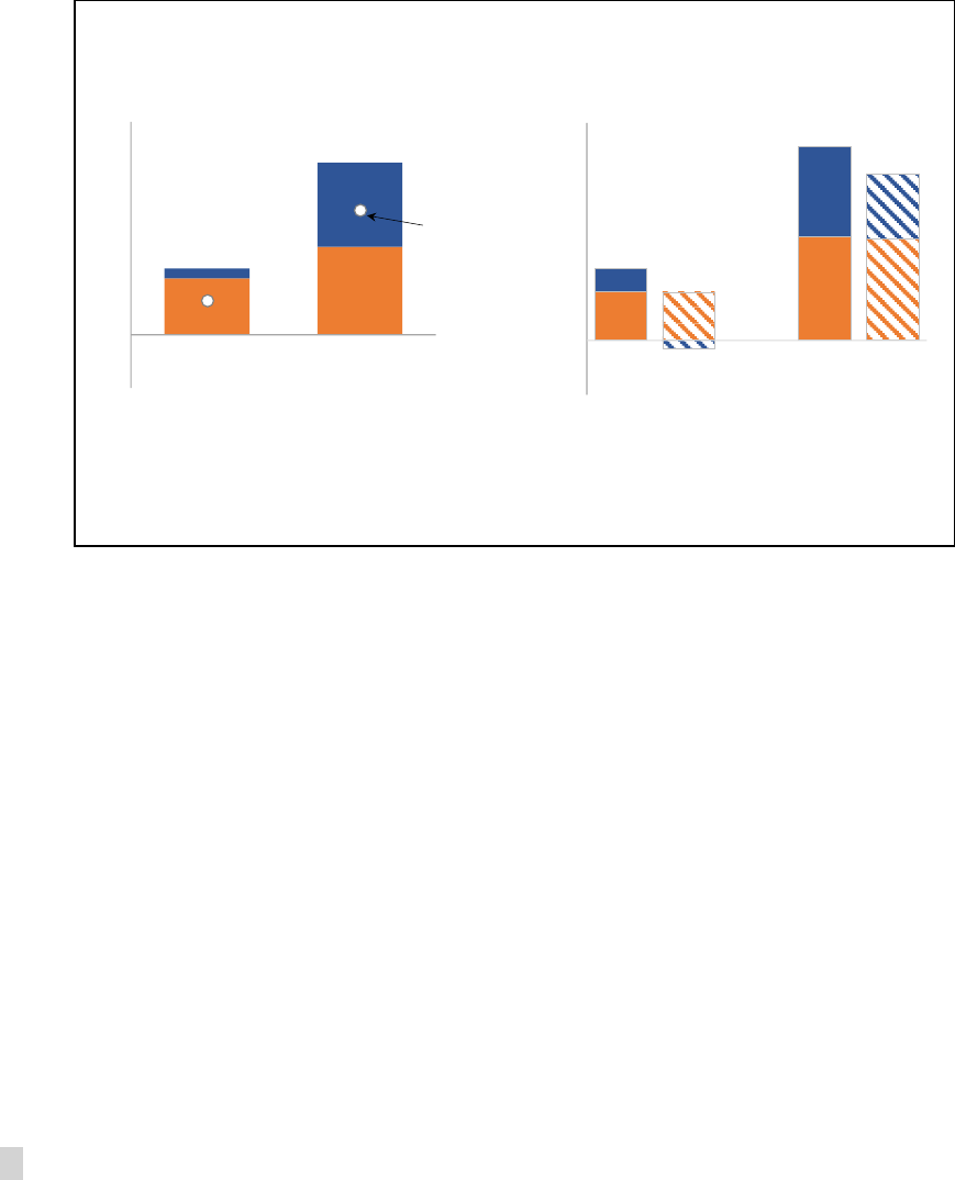
17. Dominant currency financing can shape the mechanism of exchange rates, depending on its
match (or mismatch) with the currency of trade pricing. That is, the response of trade flows to
exchange rate movements depends on the combination of pricing and financing currencies (Table 1):
19
• Producer currency pricing: If trade is priced in the currency of the producer/exporter, a depreciation
increases export volumes and reduces import volumes. This is the standard trade channel (expenditure
switching effect). So, if firms rely on local currency financing, there is no currency mismatch between
financing and revenues and, thus, the financial channel through exports is muted. In contrast,
borrowing in foreign currency entails a currency mismatch between financing and revenues, and a
depreciation tightens the financing conditions faced by exporters and importers alike, dampening the
response of export volumes and amplifying the response of import volumes, relative to the case of
local currency borrowing.
• Dominant currency pricing: In this context, exporting firms’ net revenues in US dollars are stable, while
importing firms that sell locally and therefore price in the local currency have revenues that are
volatile in US dollars. For exporters, there is no mismatch between pricing and financing currencies,
and a depreciation has a similar impact on revenues and financial costs—this is the so-called natural
hedge. Hence, the financial channel through export volumes is muted. In contrast, importers who
borrow in US dollars have a mismatch between their pricing and financing currencies, and a
depreciation can lead to tighter financial conditions and to a decline in import volumes, relative to the
case of local currency borrowing.
20
Table 1. Expected Effects of a Depreciation on Trade Volumes
Source: IMF staff.
Note: Expected effects of a depreciation of the domestic currency via-à-vis all other currencies under both PCP
and DCP are reported. DCP = dominant currency pricing; FX = foreign currency; PCP = producer currency pricing.
Thus, the financial channel reinforces expenditure switching through imports regardless of the
prevailing pricing currencies;
the effects on export volumes are, however, ambiguous under
producer currency pricing and significantly weaker
under dominant currency pricing.
B. Macro Evidence
18. While data on corporate balance sheets are limited, the available information points to
rising foreign currency liabilities, especially in emerging market economies (see Box 3). Foreign
19
Bruno and Shin (2020) explore related aspects, although they focus on the impact of global shifts of the US dollar
(vis-à-vis other currencies) through the supply of credit to emerging market firms. They focus, in particular, on the
effect through global banks’ balance sheets (as they tend to rely on US dollar funding).
20
Similar effects under dominant currency pricing and foreign currency borrowing are reported by Akinci and
Queralto (2019).
expenditure switching
(trade channel)
additional FX debt
effect
(financial channel)
expenditure switching
(trade channel)
additional FX debt
effect
(financial channel)
PCP
+ - - -
DCP
≈ 0 ≈ 0 - -
Export volumes
Import volumes

DOMINANT CURRENCIES AND EXTERNAL ADJUSTMENT
20 INTERNATIONAL MONETARY FUND
currency debt in nonfinancial firms has risen rapidly since the early 2000s, especially in emerging market
economies and following the global financial crisis—partly reflecting the low-interest-rate environment in
advanced economies (Figure 10, left panel)—although average ratios to total debt have been relatively
stable, pointing to an overall increase in indebtedness (Figure 10, right panel). Reliance on foreign
currency financing remains significantly higher in emerging market economies than in advanced
economies, even though there is significant variation within both groups (Figure 11).
Figure 10. Foreign Currency Borrowing in the Nonfinancial Corporate Sector
(US dollars and percent of total credit)
Sources: Bank for International Settlements; IMF, International Financial Statistics; and IMF staff calculations.
Note: AEs = advanced economies; EMs = emerging market economies; FC = foreign currency; NFC = nonfinancial corporate sector;
Figure 11. Foreign Currency Exposures in the Nonfinancial Corporate Sector, by Instrument, 2019
(Percent of total credit)
Sources: Bank for International Settlements; IMF, International Financial Statistics; and IMF staff calculations.
Note: In economies that host large multinational companies foreign currency exposures reflect in part the global nature of their activities.
0.0
0.1
0.2
0.3
0.4
2003q1 2005q1 2007q1 2009q1 2011q1
2013q1
2015q1 2017q1 2019q1
Average Foreign Currency Exposure
(Share of FC debt in Nonfinancial Corporate Debt)
Average AEs EMs
0.0
0.1
0.2
0.3
0.4
0.5
0
1000
2000
3000
4000
5000
6000
2003q1 2005q1
2007q1 2009q1 2011q1 2013q1 2015q1 2017q1
2019q1
Total Foreign Currency Debt in the Corporate Sector
(Million US Dollars)
AEs
EMs
EM share (right scale)
0%
20%
40%
60%
80%
CHN
IND
KOR
ISR
BRA
THA
MYS
PHL
POL
ZAF
HUN
RUS
CZE
CHL
TUR
IDN
ARG
MEX
Emerging Market Economies
0%
20%
40%
60%
80%
PRT
ITA
ESP
BEL
USA
JPN
AUT
FRA
DEU
FIN
GRC
NOR
AUS
DNK
CAN
SWE
IRL
NLD
Advanced Economies
Debt securities Loans

INTERNATIONAL MONETARY FUND 21
Box 3. Constructing Foreign Currency Debt Exposure Measures for Nonfinancial Firms
Data on the currency composition of nonfinancial corporate sector debt are scant. Although credit registries
provide direct information about the structure of borrowing at the firm level, these registries are generally available
only for a few countries and years. Macro-level data sets based on external debt statistics (for example Bénétrix,
Lane, and Shambaugh 2015), on the other hand, focus on the currency composition of external liabilities, do not
isolate the corporate sector, and abstract from local foreign currency borrowing. Two new indicators of corporate
foreign currency exposure are constructed to overcome these limitations:
1
• An indicator that follows the top-down approach of Kalemli-Ozcan, Liu and Shim (2018) and relies on the BIS
Global Liquidity Indicators database: The latter reports nonfinancial foreign currency debt held by both local
and foreign lenders on firms, government, and households. To arrive at an indicator for the nonfinancial
corporate sector, the latter measure is purged of (1) international debt securities issued by the central
government and (2) residual foreign currency loans (both cross border and local) owed by the government
and household sectors using information available in BIS Locational Banking Statistics and IMF Monetary and
Financial Statistics.
• A second indicator that follows a bottom-up approach by adding (1) foreign currency corporate debt
securities (from BIS International Debt Statistics); (2) cross-border foreign currency loans to nonfinancial firms
(from BIS Locational Banking Statistics) and (3) local foreign currency loans to nonfinancial firms (from IMF
Monetary and Financial Statistics).
The computed indicators—covering 36 major advanced and emerging market economies during 2001–19—are
used for the analysis of this section.
____________
1
See Appendix 2 for further details.
19. The macro evidence suggests that dominant currency financing amplifies the short-term
effects of exchange rates through imports. The framework presented in the section on dominant
currency financing is augmented to evaluate the effect on trade flows of a country’s currency depreciation
(vis-à-vis all other currencies) depending on the level of aggregate foreign currency borrowing.
21
As
expected, the analysis points to greater contraction in imports in response to a depreciation in importing
countries that rely more on foreign currency financing (Figure 12, panel 1). Meanwhile, the degree of
foreign currency financing in exporting countries does not appear to materially alter the effect of
exchange rates (not shown).
20. The muted effect through exports of foreign currency financing reflects the “natural
hedge” under dominant currency pricing. This is visible when comparing the estimated export volume
responses for different levels of foreign currency financing and different degrees of dominant currency
pricing (Figure 12, panel 2):
22
• When US dollar invoicing is low (producer currency pricing case) a depreciation increases exports
through the standard trade channel (because it boosts competitiveness (stand-alone effect), whereas
the effect through the financial channel is negative because the depreciation increases the burden of
US dollar debt.
21
See Appendix 3 for further details.
22
See further evidence of exporters’ natural hedge by Aguiar (2005), Du and Schreger (2016), Kalemli-Ozcan and
others (2016), and Kalemli-Ozcan (2019).

DOMINANT CURRENCIES AND EXTERNAL ADJUSTMENT
22 INTERNATIONAL MONETARY FUND
• When US dollar invoicing is high (dominant currency pricing case), by contrast, both the trade and
financial channels through exports are muted. While the depreciation improves the exporters’
competitiveness (trade
channel) and balance sheets (financial channel), export prices in US dollars
remain unchanged, as do export volumes.
Figure 12. Short-Term Trade Volume Elasticities
(Response to a 1 percent depreciation vis-à-vis all other currencies)
Source: IMF staff estimates.
Note: The bars in the left panel represent the full effect of a depreciation for different shares of foreign currency debt. All reported
estimates are significant at the 1 percent level. The right panel reports the response of export volumes for a country with a median
share of US dollar debt. Bars indicate 90 percent confidence bands. See Appendix 3 for further details on the methodology. DCP =
dominant currency pricing; FX = foreign currency; PCP = producer currency pricing.
C. Micro-Level Evidence
21. Evidence from firm-level data confirms the implications of dominant currency financing for
the mechanics of exchange rates. Available micro-level data from Colombian companies and the sharp
depreciation of the Colombian peso in 2014 provide a natural experiment to carefully identify the financial
channel of exchange rates.
23
Casas, Meleshchuk, and Timmer (2020) trace whether importing, exporting,
and the borrowing behavior of firms following the depreciation depend on the extent of pre-shock
leverage in foreign currency. The evidence shows that firms with higher foreign currency leverage
experienced significantly larger contractions in imports (Figure 13, panel 1), while there is no visible effect
of foreign currency leverage on exports. Given the high prevalence of US dollar invoicing in Colombia, the
limited impact of foreign currency leverage on exports confirms that, under dominant currency pricing,
exporters who borrow in US dollars are largely hedged. In addition, firms with higher foreign currency
leverage reduced their borrowing in foreign currency significantly more (Figure 13, panel 2)—although
they were also able to partially offset the latter with higher local currency funding—indicating the impact
23
Casas, Meleshchuk, and Timmer (2020) compile a rich data set of nearly 22,000 firms over the period 2012–17,
combining (1) firm-level data on international trade transactions from the Colombian statistical agency; (2) balance
sheet firm-level data from the Orbis global database; and (3) information on commercial loans issued by Colombian
banks from the credit registry of the Superintendencia Financiera.
-0.6
-0.4
-0.2
0.0
0.2
0.4
0.6
Stand-
alone
FX debt Combined Stand-
alone
FX debt Combined
0% USD invoicing (PCP) 100% USD invoicing (DCP)
-0.5
-0.4
-0.3
-0.2
-0.1
10th
(6.3%)
25th
(8.7%)
50th
(13.3%)
75th
(19.3%)
90th
(24.4%)
1. Short
-term import volume elasticity, by FX debt share
(response to a depreciation against all currencies)
2. Short-term export volume elasticity, by USD invocing share
(response to a depreciation against all currencies)

INTERNATIONAL MONETARY FUND 23
of balance sheet effects on the availability of financing. The evidence shows that, overall, although
exporting firms are naturally hedged, foreign currency financing exacerbates the effect of exchange rates
through imports. Moreover, the later amplification effect can be macroeconomically sizable, as illustrated
by a counterfactual exercise comparing what the import contraction would have been under hypothetical
higher and lower levels of foreign currency financing (Figure 14).
Figure 13. Effect of Foreign Currency Leverage on Firms’ Trade Flows and Borrowing
(Differential effect of one standard deviation higher foreign currency leverage)
Sources: Casas, Meleshchuk, and Timmer (2020); and IMF staff calculations.
Note: Bars depict how one standard deviation (3.2%) higher foreign currency leverage before the shock alters the impact of the
more than 50 percent depreciation of the Colombian peso vis-à-vis the US dollar on several variables during the 15 quarters
following the shock. Variables in the left panel are imports (column 1), exports (column 2), imports of firms that are not exporters
(column 3), and imports of exporting firms (column 4). Variables in the right panel are borrowing in foreign currency (column 1)
and borrowing in local currency (column 2). Column 3 depicts the implied effect on total borrowing for an average firm with non-
zero foreign currency loans before depreciation (left axis). FC = foreign currency; LC = local currency.
*** indicates statistical significance at the 99 percent level.
Figure 14. Financial Channel of Exchange Rate: Evidence from Colombia
(Import performance for various levels of foreign currency financing)
Sources: Casas, Meleshchuk, and Timmer (2020); and IMF staff calculations.
Note: The solid line depicts actual imports. The long-dashed (short-dashed) lines depict counterfactual below 0 (7) percent foreign
currency leverage. FC = foreign currency.
0.4
0.5
0.6
0.7
0.8
0.9
1.0
2012q1
2013q1
2014q1
2015q1
2016q1 2017q1
Index, 2014Q3=1
Hypothetical, no FC leverage
Hypothetical, high FC leverage
Actual
-30%
-20%
-10%
0%
10%
Imports
Exports
Imports (non-
exporters)
Imports
(exporters)
***
***
-6%
-4%
-2%
0%
2%
-60%
-40%
-20%
0%
20%
FC borrowing LC borrowing
Total borrowing
(right axis)
***
***
1. Trade Flows
2. Firm Borrowing

DOMINANT CURRENCIES AND EXTERNAL ADJUSTMENT
24 INTERNATIONAL MONETARY FUND
KEY TAKEAWAYS AND FUTURE WORK
22. The widespread use of the US dollar in trade invoicing shapes how trade flows respond to
exchange rates, leading to tepid export volume responses in the short term. This mechanism is
particularly pronounced in emerging market economies, where US dollar invoicing is more widespread.
US dollar invoicing is pervasive in manufacturing trade and also prevalent, although seemingly less so, in
services trade. Over time, the traditional exchange rate mechanism through both export and import
volumes reemerges, especially in larger economies, where US dollar pricing is less prevalent. The
dominance of the US dollar in trade invoicing also implies that a generalized shift in the value of the US
dollar vis-à-vis other currencies entails contractionary or expansionary effects on global trade and
economic activity.
23. The financing currency of firms engaged in international trade can also shape the process
of external adjustment through balance sheet effects. New analysis indicates that exposure to US
dollar borrowing has a limited impact on activities of exporting firms—which are naturally hedged in the
context of US dollar invoicing. Meanwhile, reliance on foreign currency financing amplifies the contraction
of imports in response to weakening of the domestic currency, arguably with negative effects on the
domestic economy.
24. While beyond the scope of this note, the design of optimal policies needs to take into
account the prevalence of dominant currencies for the behavior of exchange rates. With a weaker
short-term response of trade volumes to exchange rates, rebalancing external accounts or buffering the
domestic economy from macroeconomic shocks will generally require larger exchange rate movements,
and, when the latter carry adverse side effects—for example, through balance sheets or inflation—other
supportive policies may be needed. These considerations are particularly important for emerging market
and developing economies, where dominant currency pricing and financing are more common.
25. The dominance of the US dollar in trade and finance is likely to amplify the impact of the
COVID crisis. The dominance of the US dollar implies that the observed weakening of emerging and
developing countries’ currencies is unlikely to provide material boost to their economies in the short term
as the response of goods exports will be muted while some sectors that would normally respond more to
exchange rates—like tourism—are likely to be impaired by COVID-related containment measures and
consumer behavior changes. Moreover, the generalized strengthening of the US dollar may magnify the
short-term fall in global trade and economic activity as both higher domestic prices of traded goods and
services and negative balance sheet effects on importing firms contribute to lower demand for imports
throughout the emerging and developing world.
26. Tackling data gaps on invoicing and financing currencies at the firm and aggregate levels is
paramount. A key insight from the analysis is that the structure of invoicing currencies may be as
important as the composition of trading partners when it comes to measuring competitiveness in the
short term, which suggests that current indicators of competitiveness may need to be revamped or
complemented by invoicing-currency-based measures. In addition, the analysis considered the pricing
and financing currency choices as given. These decisions and their effects, however, are not independent

INTERNATIONAL MONETARY FUND 25
of one another. Thus, granular data to map pricing and financing currencies at the firm (or sector) level
are of the essence to understand the underlying market frictions that give rise to these features of
international trade and their interactions, evaluate their implications for exchange rate flexibility, and
design appropriate macroeconomic policies. Greater efforts in data collection are key to further progress
in this regard.

DOMINANT CURRENCIES AND EXTERNAL ADJUSTMENT
26 INTERNATIONAL MONETARY FUND
Appendix 1. Dominant Currency Pricing
24
When prices are sticky, the invoicing currency of cross-border transactions has significant implications for
external adjustment (that is, how trade prices and volumes react to exchange rate movements). To
illustrate this, consider a simple representation of trade flows—
—which denotes the value of trade
from country to country , measured in country ’s currency (superscript). Trade flows can be expressed
in terms of prices and quantities:
=
.
Trade prices in the exporter’s currency
(
)
can be further decomposed into the exporter’s marginal
cost in its domestic currency
(
)
and the markup
:
=
.
Under sticky prices, quantities can be assumed to be a function of prices in the currency of the destination
country (the importer)—that is, traded volumes are demand-determined—as well as some demand shock
(
):
,
.
In this setup, the effects of exchange rate changes on bilateral trade flows from to are driven (directly)
by the exchange rate pass-through to prices in the exporter’s currency (
) and (indirectly) by the pass-
through to prices in the importer’s currency (
), with the latter affecting traded quantities.
The Mundell-Fleming Framework, Producer Currency Pricing, and Local Currency Pricing
Under the Mundell-Fleming framework, the most relevant exchange rate for trade between countries
and would be their bilateral exchange rate (
). This is because the Mundell-Fleming framework does
not allow for the following:
- Product market frictions, whereby exporters may charge different markups across destination
markets (for example, due to strategic market complementarities). Hence, exporters’ markups
do not respond to exchange rate changes.
- Exporters’ use of imported intermediate inputs or decreasing marginal returns to labor: This
means that exporters’ marginal costs
(
)
do not respond to exchange rate fluctuations either.
If exporters’ markups and marginal costs do not respond to exchange rate fluctuations, the exchange rate
pass-through to prices in the exporters’ currency is zero, while the pass-through to prices in the
importers’ currency is 1. These predictions are consistent with the producer currency pricing (PCP)
paradigm, which assumes that international trade is invoiced in the currency of the exporter and that
prices in that currency are rigid. Furthermore, nominal depreciation increases the price of imports relative
to exports, thus improving competitiveness.
24
Prepared by Gustavo Adler, Sergii Meleshchuk, and Carolina Osorio Buitron. This technical appendix draws from
Chapter 2 of the 2019 External Sector Report
.

INTERNATIONAL MONETARY FUND 27
An alternative international pricing framework developed by Betts and Devereux (2000) and Devereux and
Engel (2003)—in response to evidence against the law of one price that holds under PCP—assumes that
prices are set and are rigid in the currency of the importer—so-called local currency pricing (LCP). In this
case, bilateral exchange rate movements should lead to a complete pass-through to prices in the
exporter’s currency
(
)
and zero pass-through to prices in the importer’s currency
. Hence, a
nominal depreciation increases the prices of exports relative to imports, leading to a deterioration in
competitiveness.
The Dominant Currency Pricing Framework
Recent empirical work raises questions about the validity of both PCP and LCP, showing that trade tends
to be invoiced in a small number of “dominant currencies,” with the US dollar playing a prominent role
(Goldberg and Tille 2008; Gopinath 2015), and that trade prices tend to be rigid in such currencies
(Gopinath and Rigobon 2008; Fitzgerald and Haller 2012). More recently, Casas and others (2017) and Boz,
Gopinath, and Plagborg-Møller (2018) show that, when prices are set in a third (dominant) currency ($),
trade flows between countries and are also affected by exchange rates vis-à-vis the dominant
currency (
$
and
$
). They find that the exchange rate pass-through from the dominant currency to both
export and import prices is high, while the pass-through of the bilateral (nondominant) exchange rate is
small, thus providing evidence against both PCP and LCP.
25
The authors also develop a model to explain
these phenomena: the dominant currency pricing (DCP) framework.
Building on the approach proposed by Boz, Gopinath, and Plagborg-Møller (2018) and Gopinath and
others (2020), the dominant role of the US dollar is explored by analyzing, at the country-pair level, the
relationship of traded prices and quantities to the exchange rate vis-à-vis the trading partner (
) and the
US dollar (
$
).
The framework is extended to examine the implications of DCP for the exchange rate elasticity of the
trade balance. To this end, trade prices and volumes are estimated from the perspective of both the
exporter and the importer. On the export (import) side, the focus is on the effects of a depreciation of the
exporter’s (importer’s) currency on trade volumes and prices in the exporter’s (importer’s) currency. All
these elements are necessary to compute the trade balance effect of a depreciation, for which a country-
level perspective that accounts for the exporting and importing behavior of each economy is necessary.
Specifically, while the empirical estimation focuses on trade flows between country pairs (
), the
exchange rate effect on, say, country a’s trade balance with any trading partner b is given by
=
. Summing across all trade partners yields an expression for a’s overall trade balance
response:
=
.
25
These empirical exercises can be regarded as (indirect) tests for the presence of frictions that generate exchange
rate sensitivity in markups (such as strategic pricing complementarities faced by exporters in destination markets) or
marginal costs (such as the use of imported inputs by exporting firms).
(continued)

DOMINANT CURRENCIES AND EXTERNAL ADJUSTMENT
28 INTERNATIONAL MONETARY FUND
This expression can be used to assess the impact of different exchange rate movements once the relevant
price and volume elasticities vis-à-vis the bilateral and US dollar exchange rates are estimated. Finally, the
country-level price and quantity elasticities are combined with measures of trade openness (/ and
/) to derive the response of the trade balance, as a share of output, which takes the following form:
26
=
+
.
+
$
+
$
.
$
[
…
]
,
( )
in which X/Y and M/Y denote export- and import-to-GDP ratios, respectively, and the last term on the
right side indicates a similar expression for imports to the one written in full for exports.
This general expression can be used for two thought experiments of interest:
• External adjustment: The relevant thought experiment from the perspective of correcting a country’s
external imbalance is a movement of its exchange rate vis-à-vis all other currencies. In the example
above, this would imply a shift in ’s currency vis-à-vis all other currencies, including the US dollar
(that is,
=
$
= for all ). The exchange rate between and any other country would
vary (in the same proportion), while exchange rates between any other two currencies would remain
unchanged.
• Global US dollar shifts: If prices are set in US dollars, movements in the value of this currency vis-à-vis
others would have implications for bilateral trade not only between the United States and the rest of
the world, but also among third countries. These effects can be gauged by studying the responses of
bilateral trade flows to movements in the exchange rate vis-à-vis the US dollar, while other bilateral
exchange rates remain unchanged (that is,
$
= ;
= 0 for all $).
Empirical Estimation
Building on the empirical framework of Gopinath and others (2020), the following set of equations are
estimated to obtain price and quantity elasticities for the expression above:
t
ln
=
tl
ln
+
$
tl
ln
$
+
P
×
,
+
,
;
t
ln
=
tl
ln
,
+
$
tl
ln
$
+
P
×
,
+
,
;
t
ln
=
tl
ln
+
$
tl
ln
$
+
Q
×
,
+
,
;
t
ln
=
tl
ln
+
$
tl
ln
$
+
Q
×
,
+
,
;
26
This approach abstracts from the effect of exchange rate movements on output, as the latter is of second order
importance for this analysis, for most countries.

INTERNATIONAL MONETARY FUND 29
in which ln
denotes the (log) bilateral exchange rate between the currencies of countries a and b; ln
$
is the (log) exchange rate between the currency of country a and the US dollar;
=
for
some variable , and denotes the error term. Controls include (1) country-pair fixed effects to capture
structural characteristics of any bilateral trade relationship, such as distance, common language, and so
on; (2) time fixed effects to capture global shocks that can affect trade in any given year; (3) exporters’
producer price index growth to proxy for exporters’ production costs; and (4) importers’ consumer price
index and GDP growth to capture demand shocks.
To explore short- and medium-term effects, three lags of all variables are included. Consequently, the
short-term effect of exchange rates (for example, depreciation vis-à-vis all other currencies) on the trade
balance will be given by the following:
= ×
0
+
0
$
+
0
+
0
$
×
0
+
0
$
+
0
+
0
$
.
Meanwhile, the sum of contemporaneous and lagged coefficients yields the trade balance response over
the medium term:
= ×
+
$
+
+
$
=0..3
×
+
$
+
+
$
=0..3
.
And similar expressions can be obtained for a thought experiment involving a global US dollar shift.
Data
Volumes and price indices for bilateral trade flows are obtained from the data set in Gopinath and others
(2020) based on the methodology of
Boz, Cerutti and Pugacheva (forthcoming). The data set compiles
COMTRADE data on bilateral trade at the commodity level and constructs indices for changes in volumes
and prices at the country-pair level. Bilateral exchange rates are taken from the IMF International Financial
Statistics database. Data on real GDP, real domestic demand, consumer price index, and producer price
index are taken from the IMF World Economic Outlook database.
Baseline Results
Results of the baseline specification are reported in Table A1.1. Columns 1 and 2 report exchange rate
pass-through to prices quoted in the exporter’s and importer’s currency, respectively. Columns 3 and 4
report export and import volume elasticities, respectively. Column 5 reports the effect on the trade
balance of a 10 percent exchange rate depreciation vis-à-vis all currencies, expressed in percent of GDP,
for an average country with 0.15 exports-to-GDP and imports-to-GDP ratios. The top section of the table
reports the contemporaneous coefficients—the short-term effect—and the bottom section reports the
sum of the contemporaneous and (three) lagged coefficients—which is dubbed the medium-term effect.
Coefficients for the bilateral and US dollar exchange rates are reported separately. In addition, the sum of
these two coefficients—what is called the “stand-alone” effect to distinguish it from interaction terms later
on—is reported and corresponds to the thought experiment of a depreciation vis-à-vis all trading
partners.

DOMINANT CURRENCIES AND EXTERNAL ADJUSTMENT
30 INTERNATIONAL MONETARY FUND
The baseline results correspond to the trade-weighted regressions. These provide indirect evidence of the
role of the US dollar in trade invoicing. In particular,
• The US dollar exchange rate is found to be statistically and economically significant for traded prices
and quantities in the short term. The fact that the US dollar exchange rate is relevant after controlling
for the bilateral exchange rate indicates that the US dollar is relevant for trade in country pairs that do
not include the United States.
• The export and import price coefficients on the US dollar exchange rate are symmetric, as these refer
to the same prices expressed, respectively, in the exporter’s and the importer’s currencies. Bilateral
exchange rate coefficients, however, are higher for importer currency prices than for exporter currency
prices—indicating the prevalence of producer currency pricing over local currency pricing for trade
that is not invoiced in US dollars.
• Although the importance of the US dollar remains over the medium term, the estimates of exchange
rate pass-through fall by about half, indicating that prices in the dominant currency start to adjust at
longer horizons. For trade volume elasticities, the importance of the dollar in the medium term is
negligible.
When focusing on the thought experiment of a depreciation vis-à-vis all trading partners (stand-alone
estimates), the findings are consistent with the dominant currency paradigm in the short term, while the
mechanisms of the standard Mundell-Fleming framework seem to operate over the medium term.
Specifically,
• Exchange rate pass-through to trade prices from the importer and exporter perspective is high in the
short term (0.6–0.7), indicating little variation in the terms of trade.
• Quantities display an asymmetric response in the short term. Imports fall in response to a
depreciation (vis-à-vis all currencies), indicating expenditure switching through imports.
27
This
channel is captured primarily by the US dollar exchange rate, which displays a larger coefficient than
the bilateral rate (column 3). Exports do not react because, although the bilateral exchange
rate
depreciation would
be expected to improve competitiveness and boost exports, trading partners
face the same US dollar price and thus do not change their demand for tradable goods.
27
Traditional expenditure switching through imports refers to the mechanism through which a nominal depreciation
makes foreign goods more expensive and shifts consumption toward domestically produced goods. Expenditure
switching through exports, on the other hand, implies that a nominal depreciation makes domestically produced
goods more competitive, thus boosting exports.

INTERNATIONAL MONETARY FUND 31
Table A1.1. Currency of Invoicing—Baseline Specification
(Weighted regression)
Sources: Data set from Gopinath and others (2020) and Boz, Cerutti and Pugacheva (forthcoming);
IMF, World Economic Outlook database; and IMF staff estimates.
Note: Standard errors clustered at the dyadic level are in parentheses. ER = exchange rate; FE =
fixed effects.
1/ Exporter depreciation vis-à-vis importer.
2/ Exporter depreciation vis-à-vis US dollar.
3/ Importer depreciation vis-à-vis exporter.
4/ Importer depreciation vis-à-vis US dollar.
5/ Assumed 10 percent depreciation and 0.15 openness.
***
p
< 0.01; **
p
< 0.05; *
p
< 0.1.
• While pass-through effects on prices fall somewhat over the medium term—reflecting permanent
level effects—the impact of a currency depreciation on quantities builds gradually over time.
• Furthermore, at longer horizons, the response of trade volumes is driven primarily by bilateral
exchange rate movements. This suggests that, as traded prices in the invoiced currency adjust, the
standard expenditure switching mechanism through both exports and imports reemerges.
• Taking price and quantity effects together, a 10 percent depreciation vis-à-vis all trading partners is
estimated to increase the trade balance—for a country with the average degree of trade openness—
by 0.3 percent in the short term and 1.2 percent over the medium term.
PX PM QX QM TB/Y 5/
(1) (2) (3) (4) (5)
Bi l ateral ER (exporter) 1/
0.2050*** 0.2877***
(0.0502) (0.0471)
USD ER (exporter) 2/
0.4255*** -0.2361***
(0.0333) (0.0540)
Bilateral ER (importer) 3/
0.3695*** -0.0516
(0.0527) (0.0534)
USD ER (i mporter) 4/
0.4255*** -0.2361***
(0.0333) (0.0540)
Stand-alone
0.631*** 0.795*** 0.0516 -0.288*** 0.322***
(0.0527) (0.0502) (0.0534) (0.0471) (0.102)
Bi l ateral ER (exporter) 1/
0.250*** 0.450***
(0.0401) (0.0761)
USD ER (exporter) 2/
0.256*** -0.0186
(0.0671) (0.111)
Bilateral ER (importer) 3/
0.493*** -0.432***
(0.0532) (0.0716)
USD ER (i mporter) 4/
0.256*** -0.0186
(0.0671) (0.111)
Stand-alone
0.507*** 0.750*** 0.432*** -0.450*** 1.177***
(0.0532) (0.0401) (0.0716) (0.0761) (0.186)
Observations 24,105 24,105 24,105 24,105 24,105
R-squared 0.268 0.401 0.267 0.267 0.574
Lags 3 3 3 3 3
Dyad FE YES YES YES YES YES
Year FE YES YES YES YES YES
Including USD exchange rate
Dependent variable:
Short-run elasticty
Long-run elasticty

DOMINANT CURRENCIES AND EXTERNAL ADJUSTMENT
32 INTERNATIONAL MONETARY FUND
Unweighted regressions
An alternative way of assessing cross-country differences regarding the implications of DCP for external
adjustment is by comparing the baseline estimations, in which observations are trade-weighted, with
those of an unweighted regression. The latter gives greater importance to small economies, where
invoicing in US dollars tends to be more prevalent, and as such estimates are expected to provide
stronger evidence in favor of DCP. The results of the unweighted regression are reported in Table A1.2.
Exchange rate pass-through estimates are higher than in the weighted regression, owing to the larger
coefficient on the US dollar exchange rate, at both short- and medium-term horizons. As in the weighted
regression, trade volume responses are asymmetric in the short term—negligible for exports and negative
for imports—but unlike the
trade-weighted estimates, the
asymmetry between export
and import volume elasticities
is still present over the
medium term: the export
quantity response is only one-
fourth the import volume
elasticity (in absolute value).
Despite this asymmetry, the
trade balance improves over
the medium term, and more
so than in the short term.
Degree of US dollar
invoicing
Following Boz, Gopinath, and
Plagborg-Møller (2018), data
on the share of invoicing in
US dollars are used to
examine cross-sectional
differences in exchange rate
pass-though and trade
volume elasticities for a
subsample of countries, based
on the observed degree of US
dollar invoicing. Specifically,
the implications of dominant
currency invoicing for external
adjustment are explored
directly by interacting the bilateral and US dollar exchange rates with the share of trade invoiced in US
dollars. For the price and volume equations associated with trade flows from country to country , the
relevant share of invoicing in US dollars is given by
$
, which is the GDP-weighted average of (1) the
Table A1.2. Currency of Invoicing—Unweighted Regression
(Unweighted regression)
Sources: Data sets from Gopinath and others (2020) and Boz, Cerutti and Pugacheva (forthcoming);
IMF, World Economic Outlook database; and IMF staff estimates.
Note: Standard errors clustered at the dyadic level are in parentheses. ER = exchange rate; FE = fixed
effects
1/ Exporter depreciation vis-à-vis importer.
2/ Exporter depreciation vis-à-vis US dollar.
3/ Importer depreciation vis-à-vis exporter.
4/ Importer depreciation vis-à-vis US dollar.
5/ Assumed 10 percent depreciation and 0.15 openness.
*** p < 0.01; ** p < 0.05; * p < 0.1.
PX
PM QX
QM
TB/Y 5/
(1) (2) (3) (4) (5)
Bi l a tera l ER (exporter) 1/
0.1954*** 0.3135***
(0.0140) (0.0374)
USD ER (exporter) 2/
0.5573*** -0.2695***
(0.0198) (0.0502)
Bilateral ER (importer) 3/
0.2473*** -0.0440
(0.0143) (0.0333)
USD ER (i mporter) 4/
0.5573*** -0.2695***
(0.0198) (0.0502)
Stand-alone
0.753*** 0.805*** 0.0440 -0.313*** 0.562***
(0.0143) (0.0140) (0.0333) (0.0374) (0.0897)
Bi l a tera l ER (exporter) 1/
0.256*** 0.443***
(0.0274) (0.0607)
USD ER (exporter) 2/
0.481*** -0.304***
(0.0368) (0.0870)
Bilateral ER (importer) 3/
0.264*** -0.139**
(0.0243) (0.0615)
USD ER (i mporter) 4/
0.481*** -0.304***
(0.0368) (0.0870)
Stand-alone
0.736*** 0.744*** 0.139** -0.443*** 1.055***
(0.0243) (0.0274) (0.0615) (0.0607) (0.144)
Observations 24,772 24,772 24,772 24,772 24,772
R-squared 0.532 0.586 0.149 0.149 0.328
Lags 3 3 3 3 3
Dyad FE YES YES YES YES YES
Year FE YES YES YES YES YES
Dependent variable:
Short-run elasticty
Long-run elasticty

INTERNATIONAL MONETARY FUND 33
share of country ’s exports invoiced in US dollars and (2) the share of country ’s imports invoiced in US
dollars. The following set of equations are estimated:
t
ln
=
tl
ln
+
,
tl
ln
$
+
$
ln
$
+
$,
ln
$
$
+
×
,
+
,
;
t
ln
=
tl
ln
+
,
tl
ln
$
+
$
tl
ln
$
+
$,
tl
ln
$
$
+
P
×
,
+
,
;
t
ln
=
tl
ln
+
,
tl
ln
$
+
$
ln
$
+
$,
ln
$
$
+
×
,
+
,
;
t
ln
=
tl
ln
+
,
tl
ln
$
+
$
tl
ln
$
+
$,
tl
ln
$
$
+
Q
×
,
+
,
;
in which the variables were defined previously. Under this specification, the trade balance response of a
hypothetical economy that does not have any trade invoiced in US dollars is given by the same
equations as in the baseline specification. By contrast, if the share of trade invoiced in US dollars by
economy is, on average,
$
, the short-term trade balance response is given by the following:
= ×
0
+
0
.
$
+
0
$
+ +
0
$,
$
+
0
+
0
,
$
+
0
$
+
0
$,
$
×
+
,
$
+
$
+
$,
$
+
+
,
$
+
$
+
$,
$
,
and the medium-term trade balance response is given by the sum of these coefficients up to the third lag.
Table A1.3 reports the results. The figures in black correspond to estimates for a hypothetical country for
which trade is not invoiced in US dollars. The figures in green report estimates for a country with a high
share of trade invoiced in US dollars, corresponding to the 99th percentile of the distribution (or 0.96).
The interaction terms (green coefficients) for pass-through and elasticity estimates represent the
additional effect of a high share of trade invoiced in US dollars, whereas the stand-alone green
coefficients capture the overall effect of a depreciation in such an economy.
The results confirm that the short-term external adjustment process in countries with a large share of
trade invoiced in US dollars conforms with the predictions of DCP.
• Combined pass-through estimates are high for prices of both exports and imports, as a result of the
high coefficient on the US dollar exchange rate, amounting to about 0.8, compared with an estimate
of 0.5–0.7 in economies that do not invoice in US dollars.

DOMINANT CURRENCIES AND EXTERNAL ADJUSTMENT
34 INTERNATIONAL MONETARY FUND
• Short-term trade volume elasticities in the economy that has high US dollar invoicing are
asymmetric—negligible for exports and –0.24 for imports. For the economy with no US dollar
invoicing, export and import volume elasticities are more balanced, at 0.1 and –0.2, respectively.
•
Despite the differences in the composition of external adjustment, the short-term trade balance
response is very similar across countries with different degrees of invoicing in US dollars: a 10
percent depreciation is estimated to increase the trade balance by about 0.30 percentage point
of GDP. Over the medium term, exchange rate pass-through estimates, quantity elasticities, and
trade-balance effects are quantitatively similar across countries with low and high US dollar
invoicing. Taken together, these results lend further support to the notion that dominant
currency pricing affects the composition of external adjustment mostly in the short term.

INTERNATIONAL MONETARY FUND 35
Table A1.3. Currency of Invoicing—Direct Evidence
(Weighted regression)
Sources: Data sets from Gopinath and others (2020), Boz, Cerutti and Pugacheva (forthcoming) and Boz and
others (2020); and IMF staff estimates.
Note: Standard errors clustered at the dyadic level are in parentheses. ER = exchange rate; FE = fixed effects.
*** p < 0.01; ** p < 0.05; * p < 0.1.
1/ Exporter depreciation vis-à-vis importer.
2/ Exporter depreciation vis-à-vis US dollar.
3/ Importer depreciation vis-à-vis exporter.
4/ Importer depreciation vis-à-vis US dollar.
5/ Assumed 10 percent depreciation and 0.15 openness.
PX PM QX QM TB/Y 5/
(1)
(2)
(3) (4) (5)
Bilateral ER (exporter) 1/
0.3009*** 0.2441***
(0.0360) (0.0520)
USD ER (exporter) 2/
0.2171*** -0.1276**
(0.0470) (0.0543)
Bilateral ER (exporter)*USD invoice share (99 pctile)
-0.1418*** -0.0037
(0.0457) (0.0834)
USD ER (exporter)* USD invoice share (99 pctile)
0.4443*** -0.1629*
(0.0693) (0.0928)
Bilateral ER (importer) 3/
0.4820*** -0.1165**
(0.0459) (0.0483)
USD ER (importer) 4/
0.2171*** -0.1276**
(0.0470) (0.0543)
Bilateral ER (importer)*USD invoice share (99 pctile)
-0.3025*** 0.1666**
(0.0741) (0.0735)
USD ER (importer)*USD invoice share (99 pctile)
0.4443*** -0.1629*
(0.0693) (0.0928)
Stand-alone
0.518*** 0.699*** 0.117** -0.244*** 0.330*
(0.0459) (0.0360) (0.0483) (0.0520) (0.192)
Stand-alone with USD invoice share at 99 pctile
0.806*** 0.834*** -0.0418 -0.241*** 0.314**
(0.0404) (0.0293) (0.0481) (0.0554) (0.141)
Bilateral ER (exporter) 1/
0.221*** 0.521***
(0.0509) (0.0714)
USD ER (exporter) 2/
0.198*** -0.0701
(0.0780) (0.0960)
Bilateral ER (exporter)*USD invoice share (99 pctile)
-0.0205 -0.0111
(0.0342) (0.0433)
USD ER (exporter)* USD invoice share (99 pctile)
0.268*** -0.113
(0.0649) (0.0908)
Bilateral ER (importer) 3/
0.581*** -0.451***
(0.0527) (0.0711)
USD ER (importer) 4/
0.198** -0.0701
(0.0780) (0.0960)
Bilateral ER (importer)*USD invoice share (99 pctile)
-0.248*** 0.124
(0.0636) (0.0845)
USD ER (importer)*USD invoice share (99 pctile)
0.268*** -0.113
(0.0649) (0.0908)
Stand-alone
0.419*** 0.779*** 0.451*** -0.521*** 1.126***
(0.0527) (0.0509) (0.0711) (0.0714) (0.193)
Stand-alone with USD invoice share at 99 pctile
0.667*** 0.799*** 0.326*** -0.510*** 1.295***
(0.0508) (0.0402) (0.0831) (0.0637) (0.205)
Observations
20,903 20,903 20,903 20,903 20,903
R-squared
0.500 0.688 0.343 0.343 0.569
Lags
3 3 3 3 3
Dyad FE
YES YES YES YES YES
Year FE
YES YES YES YES YES
Dependent variable:
Short-run elasticty
Long-run elasticty

DOMINANT CURRENCIES AND EXTERNAL ADJUSTMENT
36 INTERNATIONAL MONETARY FUND
Appendix 2. Measuring Foreign Currency Debt Exposure in the Nonfinancial
Corporate Sector
28
The refined measure of foreign currency debt exposure in the nonfinancial corporate sector follows the
methodology outlined in Box 2. The overall measure is available for 36 major advanced and emerging
market economies for 2001–19. Advanced economies comprise Australia, Austria, Canada, Denmark,
Finland, France, Germany, Greece, Ireland, Italy, Japan, the Netherlands, Norway, Portugal, Sweden, United
Kingdom, and the United States. Emerging market economies comprise Argentina, Brazil, Chile, China, the
Czech Republic, Hungary, India, Indonesia, Israel, Korea, Malaysia, Mexico, the Philippines, Poland, Russia,
South Africa, Thailand, and Turkey. Financial centers, such as Switzerland, Hong Kong SAR, Singapore, and
the United Kingdom, are excluded from the analysis.
Several facts are worth mentioning regarding the two indicators of foreign currency debt exposure
presented in Box 2. First, although the two measures correlate well (the correlation between the two
measures is greater than 0.8), the “top-down” approach generally yields slightly higher exposure levels
than the “bottom-up” approach. This difference stems from the fact that the top-down approach can fail
to purge noncorporate items from the total amount reported in the Bank for International Settlements
(BIS) Global Liquidity Indicators, whereas the bottom-up approach does not capture some corporate-
related items (for example, holdings of foreign currency corporate debt that are held locally). As a result,
we use an average of the two measures to generate the indicators of foreign currency exposure through
debt in the nonfinancial corporate sector depicted in Figures 11 and 12 of this Staff Discussion Note.
Second, some disaggregated components in the BIS Locational Banking Statistics and IMF Monetary and
Financial Statistics are not always available since 2001 for all countries. As a result, long time series for the
top-down indicator do not purge for residual foreign currency loans (both cross border and local) on the
government and household sectors, which are available only since 2013. Similarly, the long-time-series
version of the bottom-up approach does not include cross-border foreign currency loans to nonfinancial
corporations, which are also available only since 2013. For the regression analysis, the top-down measure
is used due to its superior coverage across time and countries, although results are robust to using
different versions (or combinations) of the two measures.
28
Prepared by Carolina Osorio Buitron and Damien Puy.

INTERNATIONAL MONETARY FUND 37
Appendix 3. The Financial Channel of Exchange Rates—Macroeconomic
Empirical Specification and Data
29
The macroeconomic empirical model builds on Gopinath and others (2020) and IMF (2019). Estimations
are conducted at the bilateral level, where each observation is composed of the observed price and
volume of a cross-border transaction between two countries. The model is extended to include exchange-
rate-induced balance sheet effects for both the exporter and importer. The following equations are
estimated as the baseline specification:
ln
=
ln
+
$
ln
$
+
,
+
,
+
×
,
+
,
; (1)
ln
=
ln
,
+
$
ln
$
+
,
+
,
+
×
,
+
,
; (2)
ln
=
ln
+
$
ln
$
+
,
+
,
+
×
,
+
,
; (3)
ln
=
ln
+
$
ln
$
+
,
+
,
+
×
,
+
,
; (4)
in which
denotes the price of a trade flow from country a to country b in the currency of the exporter
(country a);
is the price of that same trade flow in the currency of the importer (country b); Q
is
the volume of traded goods of exports from country a to country b; and
,
is a measure of
exchange-rate-induced balance sheet effects for country i at time t. The superscript X or M denotes
whether the balance sheet effect corresponds to the exporter or the importer of the transaction. Broadly
speaking, this indicator is given by
,
=
,
ln
$,
in which ln
$,
is the change in country i’s currency vis-à-vis the US dollar, and
,
is country i’s
share of foreign currency debt to total debt in the nonfinancial corporate sector.
Each equation includes the following controls:
• country-pair fixed effects to capture structural characteristics of any bilateral trade relationship, such
as distance, common language, and so on
• time fixed effects to capture global shocks that can affect trade in any given year
• exporters’ producer price index growth to proxy for exporters’ production costs
29
Prepared by Carolina Osorio Buitron and Damien Puy.

DOMINANT CURRENCIES AND EXTERNAL ADJUSTMENT
38 INTERNATIONAL MONETARY FUND
• importers’ consumer price index and GDP growth to capture, respectively, competitors’ prices and
demand shocks
The estimated equations include three lags for all variables to explore short- as well as medium-term
effects.
Data sources and definitions
Volumes and price indices for bilateral trade flows are obtained from Gopinath and others (2020). The
data set compiles COMTRADE data on bilateral trade flows at the commodity level and constructs indices
for changes in volumes and prices at the country-pair level. Bilateral exchange rates are taken from the
IMF International Financial Statistics database. Data on real GDP, real domestic demand, consumer price
index, and producer price index come from the IMF World Economic Outlook database.
The share of foreign currency debt at the country level is proxied using the top-down indicator discussed
in Box 3 thanks to its superior coverage across time and countries. Financial centers, countries that have
experienced (one or several) crises over the sample period, and large commodity exporters among
advanced economies are excluded from the sample. Finally, since exchange-rate-induced balance sheet
effects are more prominent in emerging market and developing economies, the baseline specification
relies on unweighted regressions—as opposed to trade-weighted regressions, which tend to reflect
phenomena that are more relevant for advanced economies.
Baseline results
The baseline results are reported in Table A3.1. Columns 1 and 3 report the responses of an exporter’s
depreciation on trade prices in the exporter’s currency (column 1) and trade volumes (column 3). The first
row (in black) represents the short-term (or stand-alone) effect of the exporter’s depreciation on exporter
currency prices and trade volumes—
+
$
and
+
$
,
respectively. The blue row represents
the short-term effect of the exporter’s depreciation vis-à-vis the US dollar for a median share of foreign
currency debt in total debt across exporters—
×
for exporter currency prices and
×
for traded volumes. The combined effect of the exporters’ depreciation in columns 1 and
3—that is, the stand-alone effect and the effect through exporters’ foreign currency debt exposure—is
reported in the fourth row in bold.
In a similar fashion, columns 2 and 4 show the responses of importers’ depreciation on trade prices in the
importer’s currency (column 2) and trade volumes (column 4). The first row (in black) represents the short-
term effect of the importer’s depreciation on importer currency prices and trade volumes—
+
$
and
+
$
,
respectively. The red row represents the short-term effect of the importers’ depreciation
vis-à-vis the US dollar for a median share of foreign currency debt in total debt across importers—
×
for importer currency prices and
×
for traded volumes. The combined
effect of the importers’ depreciation in columns 2 and 4 is reported in the fourth row in bold.
The upper half of the table reports the short-term (or contemporaneous) effects, whereas the bottom half
reports medium-term estimates, which correspond to the sum of the contemporaneous coefficients and

INTERNATIONAL MONETARY FUND 39
the three lags. The discussion of the results focuses on the short-term effects, since the empirical findings
suggest that currency-induced balance sheet effects are more relevant over short horizons.
The stand-alone estimates—first row of Table A3.1—are consistent with the predictions of the dominant
currency pricing framework: a depreciation is associated with high pass-through to trade prices, while
trade volumes respond to a depreciation of the importer’s currency but not a depreciation of the
exporter’s currency (see Gopinath and others, 2020, and IMF 2019). The results indicate that the
exchange-rate-induced balance sheet effects of both exporters and importers do not affect short-term
exchange rate pass-through estimates (that is, the coefficients in the second row, column 1, and third row,
column 2, are not statistically significant). Similarly, exporters’ foreign currency debt exposure does not
seem to affect trade volume elasticities (the coefficient in the second row of column 3 is not statistically
significant). An increase in the importer’s foreign debt induced by a depreciation, however, amplifies the
negative response of trade volumes (the coefficient in the third row of column 4 is negative and
statistically significant). These results are robust to estimating weighted regressions (Table A3.2) or using
alternative measures of foreign currency debt—either based on the bottom-up approach or a
combination of the top-down and bottom-up measures (not shown).
Our findings are consistent with other recent empirical literature, which has found, for emerging market
economies, that higher foreign debt exposure is related to larger import volume elasticities, whereas
exporters’ foreign debt does not seem to affect export volume elasticities (for example, Kalemli-Ozcan
and others 2016; Kalemli-Ozcan 2019).
Dollar pricing and the irrelevance of exporters’ balance sheets
The finding that exporters’ foreign currency debt exposure doesn’t affect trade volume elasticities is
associated with the “natural hedge” hypothesis. This hypothesis posits that exporters’ revenues are
denominated in US dollars and, thus, offset adverse effects of exchange rate movements through foreign
currency borrowing. In this section, we examine whether the lack of response of exporters’ foreign
currency debt is related to US dollar pricing (when exporters’ revenues are denominated in US dollars) by
including in the specification available information on both the exposure to foreign currency (US dollar)
debt as well as on US dollar invoicing shares. Specifically, to test the natural hedge hypothesis, we
compare the “combined” exchange rate response of trade volumes with a depreciation of the exporters’
currency
30
when imports in the destination country are not invoiced in US dollars with the case of
complete invoicing in US dollars. These two hypothetical cases follow mechanically from the econometric
specification, which relies on interaction terms. Specifically, the following regressions are estimated.
ln
=
ln
+
$
ln
$
+
,
+
,
+
+
ln
+
$
ln
$
+
,
+
,
+
,
(5)
30
That is, the stand-alone effect and the effect of a depreciation through the exporter’s foreign currency debt
exposure.

DOMINANT CURRENCIES AND EXTERNAL ADJUSTMENT
40 INTERNATIONAL MONETARY FUND
ln
=
ln
,
+
$
ln
$
+
,
+
,
+
+
ln
+
$
ln
$
+
,
+
,
+
,
(6)
ln
=
ln
+
$
ln
$
+
,
+
,
+
+
ln
+
$
ln
$
+
,
+
,
+
,
(7)
ln
=
ln
+
$
ln
$
+
,
+
,
+
+
ln
+
$
ln
$
+
,
+
,
+
,
(8)
The baseline specification is extended by including interaction terms with
, which measures the share of
trade invoiced in US dollars in the destination country. Exchange rates and the exporter’s foreign currency
debt exposure measure are interacted with this variable. As such, two hypothetical cases can be examined:
one in which the share of trade invoiced in US dollars is zero, the producer currency pricing (PCP) case
(
= 0), and another in which the share of trade invoiced in US dollars is 100 percent, the dominant
currency pricing (DCP) case (
= 1).
Conditional on a share of foreign currency debt, say the median share of foreign currency debt
(
), the combined exchange rate pass-through estimates into exporter and importer currency
prices under PCP are, respectively, given by the following:
+
$
=
+
$
+
×
; and
+
$
=
+
$
+
×
.
Meanwhile the trade volume elasticities to a depreciation of the importer’s and the exporter’s currencies
are, respectively, given by the following:
+
$
=
+
$
+
×
; and
+
$
=
+
$
+
×
.
In the DCP case, the effects of a depreciation of the currency of the exporter (importer) on exporter
(importer) prices are given, respectively, by the following:
+
$
=
+
$
+
+
$
+
×
+
×
; and
+
$
=
+
$
+
+
$
+
×

INTERNATIONAL MONETARY FUND 41
whereas the effects of a depreciation of the currency of the exporter (importer) on trade volumes are
given, respectively, by the following:
ln
ln
+
ln
ln
$
=
+
$
+
+
$
+
×
+
×
ln
ln
+
ln
ln
$
=
+
$
+
+
$
+
×
Table A3.3 summarizes the results. For each estimated equation, results are reported in two columns: the
PCP case (
= 0) and the DCP case (
= 1). Short-term exchange rate pass-through estimates are higher
when trade is invoiced in US dollars (columns 2 and 4) than when they are not (columns 1 and 3),
consistent with the results in Gopinath and others (2020) and IMF (2019). Further, as in the baseline
regression, the impact of exporters’ and importers’ exposure through foreign currency debt on pass-
through estimates is either economically or statistically insignificant (second row, columns 1 through 4).
Short-term trade volume elasticities to a depreciation of the exporter’s currency in the hypothetical PCP
case are reported in column 5, while column 6 provides estimates for the hypothetical DCP case. The
results for the PCP case indicate that the positive effects of a depreciation through the trade channel (first
line, column 5) are offset by the adverse effects of the depreciation through the financial channel (second
line, column 5). This result is consistent with the mechanism described in Bruno, Kim, and Shin (2018). The
authors argue that a depreciation increases exports through the trade channel—because it boosts
competitiveness—whereas the effect through the financial channel is negative—because the depreciation
tightens financial conditions. In the DCP case, by contrast, the effects of the exporter’s depreciation on
trade volumes through both the trade and financial channels are not statistically significant (first and
second rows in column 6). As explained in the conceptual framework, the DCP case results are driven by
the fact that, while the depreciation leads to an improvement in exporters’ competitiveness (trade
channel) and balance sheets (financial channel), international trade prices—which are set and are sticky in
US dollars—do not change. As a result, and given that internationally traded quantities tend to be
demand-determined, the depreciation is likely to boost exporters’ profits rather than trade volumes.
Regarding short-term trade volume elasticities to a depreciation of the importer’s currency, the results
indicate that most of the effect comes through the financial channel; that is, where importers have a larger
share of foreign currency debt, overall import volume elasticities are larger—columns 7 and 8—
irrespective of the degree of invoicing.
31
31
The result that an importer currency depreciation leads to a decline in trade volumes largely through the financial
channel (second row, columns 7 and 8), rather than the trade channel (first row, columns 7 and 8) is driven by the
sample of country pairs for which data on invoicing are available.

DOMINANT CURRENCIES AND EXTERNAL ADJUSTMENT
42 INTERNATIONAL MONETARY FUND
Table A3.1. Baseline (unweighted)
Sources: Data sets from Gopinath and others (2020), Boz, Cerutti and Pugacheva
(forthcoming), and Boz and others (2020); and IMF staff estimates.
Note: Robust standard errors reported in parentheses. ER = exchange rate; FX = foreign
currency; FE = fixed effects. *** p < 0.01; ** p < 0.05; * p < 0.1.
Table A3.2. Weighted Regressions
Sources: Data sets from Gopinath and others (2020), Boz, Cerutti and Pugacheva
(forthcoming), and Boz and others (2020); and IMF staff estimates.
Note: Robust standard errors are reported in parentheses. ER = exchange rate; FX =
foreign currency; FE = fixed effects. *** p < 0.01; ** p < 0.05; * p < 0.1.
PX PM QX QM
(1) (2) (3) (4)
ER elasticty 0.649*** 0.753*** 0.0557 -0.122*
(0.0379) (0.0351) (0.0691) (0.0658)
FX debt * USD ER (exporter) -0.00138 -0.0517
(0.0376) (0.0652)
FX debt * USD ER (importer) 0.0454 -0.161**
(0.0370) (0.0661)
Combined effect 0.647*** 0.799*** 0.00401 -0.282***
(0.0309) (0.0281) (0.0567) (0.0533)
ER elasticty 0.561*** 0.795*** 0.499*** -0.438***
(0.0616) (0.0595) (0.133) (0.113)
FX debt * USD ER (exporter) -0.0113 -0.224*
(0.0492) (0.120)
FX debt * USD ER (importer) 0.0420 -0.124
(0.0578) (0.105)
Combined effect 0.550*** 0.837*** 0.276*** -0.562***
(0.0500) (0.0559) (0.101) (0.0963)
Observations 8,674 8,674 8,674 8,674
R-squared 0.264 0.278 0.243 0.243
Lags 3 3 3 3
Dyad FE YES YES YES YES
Year FE YES YES YES YES
Dependent variable:
Short-run
Medium-run elasticty
PX PM QX QM
(1) (2) (3) (4)
ER elasticty 0.631*** 0.649*** 0.0296 -0.148**
(0.0712) (0.0592) (0.0633) (0.0699)
FX debt * USD ER (exporter) 0.00279 0.00444
(0.0118) (0.00713)
FX debt * USD ER (importer) 0.0839*** -0.127**
(0.0321) (0.0540)
Combined effect 0.634*** 0.733*** 0.0340 -0.275***
(0.0614) (0.0461) (0.0596) (0.0523)
ER elasticty 0.583*** 0.647*** 0.238** -0.271**
(0.0788) (0.0786) (0.103) (0.120)
FX debt * USD ER (exporter) -0.000724 0.0131
(0.00907) (0.0149)
FX debt * USD ER (importer) 0.0611 -0.181**
(0.0462) (0.0765)
Combined effect 0.582*** 0.708*** 0.251*** -0.452***
(0.0734) (0.0735) (0.0962) (0.101)
Observations 8,674 8,674 8,674 8,674
R-squared 0.341 0.370 0.484 0.484
Lags 3 3 3 3
Dyad FE YES YES YES YES
Year FE YES YES YES YES
Dependent variable:
Short-run
Medium-run elasticty

INTERNATIONAL MONETARY FUND 43
Table A3.3. Estimates by US Dollar Invoicing Share
Sources: Data sets from Gopinath and others (2020), Boz, Cerutti and Pugacheva (forthcoming), and Boz and others (2020); and IMF staff estimates.
Note: Robust standard errors are reported in parentheses. ER = exchange rate; FXD = foreign currency debt; FE = fixed effects. *** p < 0.01; ** p < 0.05;
* p < 0.1.
importer USD invoicing:
S=0
S=1 S=0
S=1 S=0
S=1
S=0 S=1
(1)
(2)
(3)
(4)
(5)
(6) (7) (8)
Stand-alone ER elasticty 0.596***
0.753*** 0.757***
0.764*** 0.191*
-0.111 -0.143 0.182*
(0.0582) (0.0844) (0.0577) (0.0491)
(0.115)
(0.127) (0.124)
(0.105)
Currency induced FXD effect 0.0273 -0.0845 0.00850 0.00850 -0.250**
0.189 -0.300***
-0.300***
(0.0625)
(0.0966)
(0.0353) (0.0353)
(0.121)
(0.126) (0.0792) (0.0792)
Combined effect
0.623***
0.668*** 0.765***
0.772***
-0.0588 0.0778
-0.443*** -0.118
(0.0487) (0.0579)
(0.0525) (0.0454)
(0.0917) (0.104)
(0.119)
(0.0945)
Stand-alone ER elasticty 0.521*** 0.602*** 0.662*** 0.819***
0.605*** 0.445*
0.115 -0.674***
(0.0975)
(0.0890)
(0.0945) (0.0825) (0.209)
(0.228) (0.192)
(0.181)
Currency induced FXD effect 0.0398 -0.121 -0.0387
-0.0387
-0.332 -0.0746
-0.124 -0.124
(0.0866) (0.0920) (0.0568) (0.0568)
(0.229) (0.221)
(0.114) (0.114)
Combined effect 0.560*** 0.481*** 0.624*** 0.780*** 0.273 0.371** -0.00926 -0.798***
(0.0808) (0.0876) (0.104) (0.0731)
(0.181)
(0.164) (0.205) (0.135)
Observations
R-squared
Lags
Dyad FE
Year FE
YES
YES
YES
YES
YES
YES
YES
YES
0.299
0.260
0.307
0.260
3
3
3
3
7,511
Dependent variable:
PX
(equation 5)
PM
(equation 6)
QX
(equation 7)
QM
(equation 8)
Short-run
Long-run
7,511
7,511
7,511

DOMINANT CURRENCIES AND EXTERNAL ADJUSTMENT
44 INTERNATIONAL MONETARY FUND
REFERENCES
Adler, Gustavo, Sergii Meleshchuk, and Carolina Osorio-Buitron. 2019. “Global Value Chains and External
Adjustment: Do Exchange Rates Still Matter?” IMF Working Paper 19/300, International Monetary
Fund, Washington, DC.
Aguiar, Mark. 2005. “Investment, Devaluation, and Foreign Currency Exposure: The Case of Mexico.”
Journal of Development Economics 78:95–113.
Akinci, Ozge, and Albert Queralto. 2019. “Exchange Rate Dynamics and Monetary Spillovers with Imperfect
Financial Markets." Federal Reserve Bank of New York Staff Reports.
Amiti, Mary, Oleg Itskhoki, and Jozef Konings. 2014. "Importers, Exporters, and Exchange Rate
Disconnect." American Economic Review 104 (7): 1942–78.
Amiti, Mary, Oleg Itskhoki, and Jozef Konings. 2018. “Dominant currencies: How firms choose currency
invoicing and why it matters,” Technical Report, National Bank of Belgium Working Paper No. 353.
Bénétrix, Agustin S., Philip R. Lane, and Jay C. Shambaugh. 2015. "International Currency Exposures,
Valuation Effects and the Global Financial Crisis." Journal of International Economics 96 (S1): S98–S109.
Bernard, Andrew B., J. Bradford Jensen, and Peter K. Schott. 2009. Importers, Exporters and Multinationals:
A Portrait of Firms in the US that Trade Goods. NBER Chapters, pp.513-552.
Betts, C., and M. Devereux. 2000. “Exchange Rate Dynamics in a Model of Pricing-to-Market.” Journal of
International Economics 50 (1): 215–44.
Bils, Mark, and Peter J. Klenow. 2004. “Some Evidence on the Importance of Sticky Prices.” Journal of
Political Economy 112 (5): 947–85.
Boz, Emine, Camila Casas, Georgios Georgiadis, Gita Gopinath, Helena Le Mezo, Arnaud Mehl and Tra
Nguyen, 2020, “Invoicing Currency Patterns in Global Trade” IMF Working Paper, International
Monetary Fund, Washington DC
Boz, Emine, Eugenio Cerutti and Evgenia Pugacheva. Forthcoming. “Dissecting the Global Trade
Slowdown: A New Database.” IMF Working Paper, International Monetary Fund, Washington, DC.
Boz, Emine, Gita Gopinath, and Mikkel Plagborg-Møller. 2018. “Global Trade and the Dollar," Harvard
University, Cambridge, MA.
Bräuning, Falk, and Victoria Ivashina. 2017. “Monetary Policy and Global Banking.” NBER Working Paper
23316, National Bureau of Economic Research, Cambridge, MA.
Bruno, Valentina, Se-Jik Kim, and Hyun Shin. 2018. "Exchange Rates and the Working Capital Channel of
Trade Fluctuations." AEA Papers and Proceedings 108:531–36.
Bruno, Valentina, and Hyun Shin. 2020. "Dollar and Exports." BIS Working Paper 819, Bank for
International Settlements, Basel.
Casas, Camila, J. Federico Diez, Gita Gopinath, and Pierre-Olivier Gourinchas. 2017. “Dominant Currency
Paradigm: A New Model for Small Open Economies.” IMF Working Paper 17/264, International
Monetary Fund, Washington, DC.
Casas, Camila, S. Meleshchuk, and Y. Timmer. 2020. “The Dominant Currency Financing Channel of
External Adjustment.” Banco de la Republica de Colombia. Borradores de Economía; No. 1111.

INTERNATIONAL MONETARY FUND 45
Devereux, Michael, and Charles Engel. 2003. "Monetary Policy in the Open Economy Revisited: Price
Setting and Exchange Rate Flexibility." Review of Economic Studies 70:765–84.
Du, Wenxin and Schreger, Jesse. 2016. “Sovereign Risk, Currency Risk, and Corporate Balance Sheets,”
Harvard Business School BGIE Unit Working Paper No. 17-024.
Fitzgerald, Doireann, and Stefanie Haller. 2012. “Exchange Rates and Producer Prices: Evidence from Micro
Data.” Working Paper, Stanford University, Stanford, CA.
Francois, Joseph, and Bernard Hoekman. 2010. "Services Trade and Policy." Journal of Economic
Literature 48 (3): 642–92.
Francois, Joseph, and Olga Pindyuk. 2013. "Consolidated Data on International Trade in Services." IIDE
Discussion Paper 20130101, Institute for International and Development Economics, Rotterdam.
Friberg, Richard and Wilander, Fredrik (2008). “The currency denomination of exports – a questionnaire
study.” Journal of International Economics, 75 (1): 54–69.
Gabaix, Xavier, and Matteo Maggiori. 2015. “International Liquidity and Exchange Rate Dynamics,"
Quarterly Journal of Economics 130 (3): 1369–420.
Goldberg, Linda S. and Cédric Tille. 2008. “Vehicle Currency Use in International Trade.” Journal of
international Economics 76 (2): 177–92.
———. 2016. “Micro, Macro, and Strategic Forces in International Trade Invoicing: Synthesis and Novel
Patterns.” Journal of International Economics 102:173–87.
Goldberg, Pinelopi Koujianou, and Rebecca Hellerstein. 2008. "A Structural Approach to Explaining
Incomplete Exchange-Rate Pass-Through and Pricing-to-Market." American Economic Review 98 (2):
423–29.
Gopinath, Gita. 2015. “The International Price System.” Technical Report, National Bureau of Economic
Research, Cambridge, MA.
———, and Roberto Rigobon. 2008. “Sticky Borders.” Quarterly Journal of Economics 123 (2): 531–75.
Gopinath, Gita, Oleg Itskhoki, and Roberto Rigobon. 2010. “Currency Choice and Exchange Rate Pass-
through.” American Economic Review 100 (1): 304–36.
Gopinath, Gita, and Jeremy C. Stein. 2018. “Banking, Trade, and the Making of a Dominant Currency."
Harvard and NBER paper, Harvard and National Bureau of Economic Research, Cambridge, MA.
Gopinath, Gita, Emine Boz, Camila Casas, Federico Diez, Pierre-Olivier Gourinchas, and Mikkel Plagborg-
Møller. 2020. “Dominant Currency Paradigm.” American Economic Review 110 (3): 677-719.
Hoekman, Bernard, and Ben Shepherd. 2019. “Services Trade Policies and Economic Integration: New
Evidence for Developing Countries,” No. 14181. CEPR Discussion Papers.
International Monetary Fund (IMF). 2019. External Sector Report, Chapter 2. Washington, DC.
Kalemli-Ozcan, Sebnem. 2019, “U.S. Monetary Policy and International Risk Spillovers.” Jackson Hole
Symposium, Jackson Hole, WY.
Kalemli-Ozcan, S, X Liu and I Shim. 2018. "Exchange rate appreciations and corporate risk taking," BIS
Working Papers no 710

DOMINANT CURRENCIES AND EXTERNAL ADJUSTMENT
46 INTERNATIONAL MONETARY FUND
Klenow, Peter J., and Benjamin A. Malin. 2010. “Microeconomic Evidence on Price-Setting” Handbook of
Monetary Economics, vol. 3, 231–84. Amsterdam: Elsevier.
Kugler, Maurice and Eric Verhoogen. 2009. “Plants and imported inputs: New facts and an interpretation,”
American Economic Review, 99(2), 501–07.
Lane, Philip R., and Jay C. Shambaugh. 2010. “Financial Exchange Rates and International Currency
Exposures.” American Economic Review 100 (1): 518–40.
Li, Nan, and Sergii Meleshchuk. Forthcoming. “Exchange Rates and Services Trade Flows: The Evidence of
Dominant Currency.” IMF Working Paper, International Monetary Fund, Washington, DC.
Manova, Kalina and Zhiwei Zhang. 2009. “China’s exporters and importers: Firms, products and trade
partners,” Technical Report, National Bureau of Economic Research.
Mukhin, D., 2018. “An Equilibrium Model of the International Price System,” mimeo.
