Invoicing Currency Choice: Strategic Complementarities and

Invoicing Currency Choice:

Strategic Complementarities and Currency Matching

Yushi Yoshida

∗ a f

, Junko Shimizu

b f

, Takatoshi Ito

c f

, Kiyotaka Sato

d f

Taiyo Yoshimi

e f

, and Uraku Yoshimoto

Shiga University

Gakushuin University

Columbia University and NBER

Yokohama National University

Chuo University

Policy Research Institute, Ministry of Finance

January 5, 2024

Abstract

Japanese exporters’ choice of invoice currencies is investigated using newly available of-

ﬁcial Customs declaration data, which records detailed information, including the trading

partners’ names, invoicing currency, and product descriptions. The strategic complementar-

ity mechanism, that is, choosing the same invoice currency as others in the same industry or

the same destination market, is found among Japanese exporters. We propose the “broad

two-way exporters” whose export destinations and import origins do not necessarily match

and the “narrow two-way exporters” whose export destination and import origins match in

the same year. It is found that currency matching for exports and imports is as essential as

strategic complementarity for two-way exporters. However, as one of this paper’s novelty,

we found evidence that newly entering two-way exporters are less concerned about currency

matching. Therefore, the currency matching mechanism for two-way exporters is gradually

formed as they continue to survive in international markets.

∗

corresponding author: yushi.yoshida@biwako.shiga-u.ac.jp. This study is the result of research conducted

jointly with the Policy Research Institute (PRI), which submitted an oﬀer of use to the Ministry of Finance based

on the “Guideline on the utilization of Customs’ import and export declaration data in a joint research with Policy

Research Institute,” and received approval in February 2022. The views expressed in this research are those of the

author’s personal responsibility and do not represent the oﬃcial views of the Ministry of Finance or the Policy

Research Institute of the Ministry of Finance. The authors thank the staﬀ at the PRI for the great research

support they received, especially Kenta Ando, Fumiharu Ito, and Shintaro Negishi, for the use of transaction-

level microdata. We especially thank Wanyu Chung, Rob Elliott, and Kazunobu Hayakawa for their insightful

comments on the earlier version of this paper, and we also thank the participants in the research meetings at the

PRI, universit´e Sud Bretagne, University of Birmingham, ETSG conference at the University of Surry, French-

Japanese Webinar, and JSME conference at Kyushu University for their useful comments. Yoshida gratefully

acknowledges ﬁnancial support from the JSPS KAKENHI 20H01518, 22K18527, and 23H00836. Shimizu, Sato,

Yoshimi, and Yoshimoto thank 18K01698, 23H00836 & 23K17550, 20H01518 & 20KK0289, and JP21K20172, for

ﬁnancial support, respectively.

Keywords: Currency Matching; Customs Data; Dominant Currency; invoicing currency;

Strategic Complementarities.

JEL Classiﬁcation: F14; F31; F61.

1 Introduction

In addition to making decisions for producing and distributing their products to foreign cus-

tomers, exporters must choose the invoicing currency for their exports. Faced with ﬂuctuating

exchange rates, the choice of invoicing currency aﬀects the exporter’s revenue in terms of home

currency, as discussed in Gopinath and Rigobon (2008) and Gopinath, Itskhoki, and Rigobon

(2010).

This study investigates determinants of invoicing currency choice by utilizing the ex-

port/import transaction level data at Japan Customs that have become available recently. Each

transaction entry includes the identiﬁcation of the exporter/importer, the departing/landing

port, the content of products, invoicing currency, volume, value, the identiﬁcation of the trading

partner, the port in the partner’s country, mode of transport, and other detailed information

regarding exporting and importing.

Instead of working on individual raw transaction records, we aggregated transaction records

by pairs of exporters and trading partner countries. The choice of the aggregation strategy

makes us depart from the existing studies in the literature. The aggregation of granular data is

not usually pursued in research simply because of fear of losing information and the number of

observations. However, the beneﬁts of some aggregation outweigh the cost. Invoicing currency

decisions at the granular level are not independent of each other.

The choice of invoice currency will depend on the destination countries. For example, the

exporter is more likely to choose US dollar invoicing for exports to the United States while

choosing the British Pound for exports to the United Kingdom. These considerations lead us to

work on the pairs of exporters and trading partner countries. Moreover, there will be no loss of

observations, as the aggregation still leaves the data set with three million transaction records

of exports for seven years between 2014 and 2020, as shown in Table 2.

Using the Belgian ﬁrm transaction level data, Amiti, Itskhoki, and Konings (2022) showed the

phenomenon called strategic complementarity, i.e., the competitors’ choice of invoicing currency

in the same industry and market induces an exporter to choose the same currency.

Following

Gopinath, Itskhoki, and Rigobon (2010) and Amiti, Itskhoki, and Konings (2022), we examine

whether Japanese exporters choose invoicing currency with consideration of strategic comple-

The choice of invoicing currency also has a macroeconomic consequence for the importing country. If a large

portion of the import is invoiced in the importing country’s currency, i.e., local currency pricing, the import price

index shows a small change with respect to a change in the exchange rate. In contrast, invoiced in the exporter’s

currency, i.e., producer currency pricing, the import price index demonstrates a relatively large proportionate

change.

Amiti, Itskhoki, and Konings (2019) deﬁne strategic complementarity in terms of the elasticity of own price

to a change in the competitors’ price.

mentarities, that is, to select the same invoicing currency as their competitors. For exporters

facing competition from other ﬁrms, setting their prices to move in tandem with competitors’

prices is essential. For example, Japanese exporters use the US dollar as invoicing currency

because their competitors also use US dollar invoicing in the same destination country and/or

in the same industry. Amiti, Itskhoki, and Konings (2022) constructed strategic complemen-

tarity variables at the industry-destination level. However, they did not diﬀerentiate exports

by destination or by industry. We investigate which one of the destination countries or which

industry factor puts more pressure on an exporter’s choice of invoice currency. The country-

speciﬁc strategic complementarity variable is the ratio of all other ﬁrms’ exports invoiced in the

US dollar to the overall export value of all other ﬁrms in the destination country. The industry-

level strategic complementarity variable is constructed in two steps. First, we construct the US

dollar ratio in each HS 4-digit industry by all other ﬁrms to all destination countries. Second,

the weighted average of US dollar ratios at HS 4-digit industries, with weight being the share of

ﬁrms’ exports in the industry over the ﬁrm’s total exports.

In addition, we also ﬁnd that exporters tend to choose the invoicing currency for exports to

match the invoicing currency for their imports. Previous studies in the literature found such

a link. Chung (2016) ﬁnds that using producer currency for inputs increases the likelihood of

UK exporters choosing local currency for exports. As in other authors, the observation unit

in Chung (2016) is ﬁrm-product-destination. We generalize the concept and broaden it to the

ﬁrm-destination level. The Japanese exporters favor using US dollar invoicing in exports to

a destination if their imports from the same country are invoiced in US dollars. This is not

only so for the case of dominant currency but also applies to the cases of producer currency

pricing and local currency invoicing. With this data set, we deﬁne narrow two-way exporters as

exporters that export to and import from the same country.

Among determinants of invoicing

currency choice, we found that currency matching is as essential as strategic complementarity

for exporters who do imports and exports. By matching the invoice currency for exports with

that for imports, the exporter can minimize the exchange risk generated by currency mismatch.

Our contribution is sixfold. First, this study is one of the ﬁrst to use the Japan Customs

transaction data, which have only recently become available for select researchers. The avail-

ability of transaction-level data with information on currency invoicing made it possible for us to

push forward the research on invoicing currency choice for Japanese exporters. Some countries

have inherent problems in investigating the issue of invoicing currency choice. The US dollar

is simultaneously the dominant and local currency for US imports, as argued in (Gopinath and

In the empirical section, we propose narrowly deﬁned and broadly deﬁned two-way exporters.

Rigobon 2008); therefore, it is impossible to distinguish between the eﬀects of local and dominant

currency. A particular problem arises for EU member countries: No information on invoicing

currency is recorded at the Customs oﬃce because intra-EU trade is exempt from customs. The

Belgian exporters use the euro extensively with neighboring countries

; thus, excluding these ex-

ports from the analysis may distort the results(Amiti, Itskhoki, and Konings 2022), reducing the

sample size signiﬁcantly. Since the U.K. is not in the Eurozone, the UK data seem to have fewer

similar problems, as shown in Chung (2016),Crowley, Han, and Son (2021),Corsetti, Crowley,

and Han (2022).

Therefore, investigating the exporters with their home currency being neither

the dollar nor the euro is expected to make an important contribution to the literature.

Using

the new data set for Japanese ﬁrms, we examine how dollar invoicing is used for non-dollar des-

tination countries without discarding a large portion of trade data, unlike some previous studies

in the literature.

Second, the primary variable of analysis is the ﬁrm-destination pair. Instead of using raw

transaction data, we aggregated the data at the level of exporting ﬁrms and destination coun-

tries. In this way, we can capture the exporters’ motive for the common invoicing currency,

i.e., the cost of managing multiple currencies can be avoided. More formally, the decisions on

invoicing currency are not independent among transactions, at least for those under the same

macroeconomic environment, i.e., exports to the same destination country. We are aware of the

trade-oﬀ between the beneﬁt of aggregation and the loss of detailed information. The optimal

level of aggregation for investigating the choice of invoicing currency depends on the objective

of the research. We believe that using a ﬁrm-destination pair in this study brings forth several

advantages without signiﬁcant loss of information in the original dataset. We assume that ﬁrms

make an invoicing currency decision at the partner country level, not at each transaction level.

Theoretical models in the literature, for example, Amiti, Itskhoki, and Konings (2022) assume

that a ﬁrm sells only one product to one market. In this case, the solution to the ﬁrm’s optimiza-

tion problem leads to a uniquely chosen single currency. However, in reality, a ﬁrm tends to sell

many products to the same market. The ﬁrm’s optimal decision would not be a single currency

for exports for all products. Diﬀerent products may have diﬀerent invoicing currencies. The

choice of a product is aﬀected by each product’s idiosyncratic sensitivity of marginal cost and

In 2018, non-EU destination exports (imports) by Belgian ﬁrms made up only 27 (34) percent of total exports

(imports), (Amiti, Itskhoki, and Konings 2022). However, Boz, Casas, Georgiadis, Gopinath, Le Mezo, Mehl,

and Nguyen (2022) demonstrate that assuming the use of the euro being 100 percent within the Euro area is not

plausible.

In 2011, non-EU destination exports by UK ﬁrms accounted for 46.5% of the total UK exports, (Chung 2016).

The strong presence of the Japanese yen in foreign exchange markets also makes it interesting. The Japanese

yen as an invoicing currency is relatively more acceptable by trading partners than minor currencies.

markup to foreign currencies. Our empirical analysis shows that the ﬁrm’s invoicing currency

decisions are well explained at the ﬁrm-country pair level.

Third, we provide two decomposed dimensions of strategic complementarity: destination

country and industry. The existing studies, such as Amiti, Itskhoki, and Konings (2022), measure

strategic complementarity at the ﬁrm- industry-country level. The index at this level correctly

captures the interaction among the Belgian exporters, but distinguishing the diﬀerence among

destinations is not measured. We constructed a strategic complementary index based on the

destination country, i.e., how much other Japanese exporters use US dollars as an invoicing

currency given the destination country. The other index based on industry is more complicated

because we use ﬁrm-level instead of single transaction as a unit of observations. As a preliminary

step, we construct the US dollar ratio as an invoicing currency for each HS 4-digit industry. Then,

we calculate a weighted US dollar ratio by other exporters with weights as industry proportions

of an exporter’s exports. We ﬁnd that the positive eﬀects of both dimensions of strategic

complementarity are statistically signiﬁcant and robust to any speciﬁcations. The magnitude

of strategic complementarity at the industry dimension is signiﬁcantly larger. Therefore, the

invoicing currency choice is driven more by which industry an exporter competes in than where

it competes.

Fourth, two deﬁnitions of two-way exporters are proposed considering the matching of invoic-

ing currencies between exports and imports. broad two-way exporters are deﬁned as those who

export and import, with destination and origin may not be the same. Narrow two-way exporters

are deﬁned as those who export to and import from the same country. We ﬁnd that narrow

two-way exporters are more inclined to match invoicing currencies of exports and imports than

broad two-way exporters.

Fifth, we adopt a fractional probit regression with instrumental variables. In the previous

studies examining the invoicing currency choice at the transaction level, probit or logit models

were applied to the binary dependent variable of taking the value of one if the target currency

is chosen and zero otherwise. We apply the fractional probit estimation method because the

invoicing currency ratio ranges between zero and one.

Sixth, we also examine the invoicing currency choice of ﬁrms newly entering export markets.

The panel estimates may suﬀer from biased estimates because currency invoicing decisions are

persistent. Long-surviving ﬁrms may only repeatedly use the same currency as the previous

years. In order to capture the ﬁrst decision of choosing invoicing currency, new entrants that

did not engage in any international trade in the last year are free from such a bias. The currency

matching motive is less pursued, whereas the strategic complementarity motive is essential from

the ﬁrst year.

The rest of this paper is organized as follows. The next section describes how the data set

is prepared in this study. Section 3 provides empirical models, and section 4 shows empirical

evidence. Section 5 revisits the invoicing currency choice of new exporters, and the last section

concludes.

2 Invoicing Currency Choice at the Firm-Country level

2.1 The Export and Import Declarations submitted to the Japan Customs

Oﬃce

The data set became available in 2022 under a program of government-owned data utilization

at the Ministry of Finance, Japan.

The data consists of a complete set of general export and

import declarations between 2014 and 2020.

Each transaction is recorded as a separate record,

even for the same ﬁrm, and the number of records for exports is in the order of millions for one

year. Table 1 summarizes this dataset between 2014 and 2020 by invoicing currency.

The left part of Table 1 provides the statistical summary of this export data set. On the

top row, with the total export values at the leftmost, the ratios of invoicing currencies are

shown. Four currencies of interest are (i) the Japanese yen, the producer currency for Japanese

exporters; (ii) the US dollar, the dominant currency of the world; (iii) the euro, the largest

regional currency in Europe; and (iv) local currencies, i.e., the oﬃcial national currency used in

the destination country. US dollars have the largest share, 51 percent, in the invoicing currency

of Japanese exports. The Japanese yen is also extensively used for 36 percent of the invoiced

currency in Japanese exports, but the euro plays a small part as it is only 6 percent of Japan’s

exports. The seemingly high ratio of local currency invoicing can be explained using the US

dollar in the US and the Euro in the Euro area.

Panel A of Table 1 shows the use of invoicing currencies by country and region. The US

dollar is overwhelmingly used in exports to the US market, and it is also the largest invoicing

currency in China and the rest of Asia. Although a small share in overall trade, Euro invoicing

is signiﬁcant at 56 percent in the Euro area.

For the rest of the world, excluding the US and

Euro area, the local currency invoicing is below six percent, not shown in the table.

Researchers aﬃliated with universities need to be cross-appointed by the Ministry of Finance and work under

the binding regulations of public oﬃcers. Any private information revealed to the researchers during the research

must be kept secret.

Low-value cargoes under the simpliﬁed customs clearance are excluded from the database.

The countries included in the Asia and Euro area are listed in the appendix.

Panel B of Table 1 shows invoicing currency for selected industries. The overall picture does

not change much; however, the Japanese yen is the most-used invoicing currency in the textile

industry, and the US dollar use is even ampliﬁed to 68 percent in the base metal industry. The

right part represents the invoicing currency for imports. Like exports, the US dollar is also

the dominant invoicing currency in Japanese imports. The use of the US dollar is even more

pronounced in imports, 61 percent. The noteworthy facts are that 71 percent of imports from

China are invoiced in the US dollar, and textile imports are invoiced in the currency of the

exporting country for only ﬁve percent.

Table 1: Invoice currency by region and industry (2014-2020)

Exports Imports

values JPY (PCP) USD EUR LC values JPY (LCP) USD EUR PC

ALL 552 0.36 0.51 0.06 0.27 563 0.32 0.61 0.04 0.14

Panel A: by trading regions values JPY (PCP) USD EUR LC values JPY (LCP) USD EUR PC

US 105 0.13 0.87 0.00 0.87 61 0.25 0.74 0.01 0.74

Euro Area 46 0.32 0.12 0.56 0.56 55 0.53 0.11 0.33 0.33

China 136 0.42 0.52 0.00 0.06 138 0.24 0.71 0.01 0.04

ASIA 167 0.47 0.47 0.00 0.05 133 0.38 0.58 0.00 0.03

Panel B: by HS sections values JPY (PCP) USD EUR LC values JPY (LCP) USD EUR PC

Chemical (Sec.6) 44 0.33 0.57 0.05 0.20 47 0.54 0.38 0.04 0.16

Textiles (Sec.11) 7 0.48 0.45 0.05 0.12 29 0.16 0.79 0.03 0.05

Base Metal (Sec.15) 46 0.26 0.68 0.03 0.13 28 0.37 0.57 0.03 0.13

Machinery & Electronics (Sec.16) 204 0.41 0.47 0.07 0.24 134 0.25 0.67 0.05 0.16

Transport (Sec.17) 127 0.31 0.50 0.08 0.48 23 0.50 0.31 0.14 0.25

Precision Instruments (Sec. 18) 35 0.35 0.49 0.09 0.29 25 0.43 0.41 0.07 0.28

Note: The ﬁgures in the ﬁrst column (values) represent the total export values in trillion Japanese yen between 2014 and 2020.

The ﬁgures in other columns represent the ratio of invoice currency used in the corresponding region/sectors. LC and PC are

trade partners’ currencies. LC in exports represents local currency invoicing, and PC in imports represents producer currency

invoicing. Asia region includes 21 countries, excluding China. The number of countries in the Euro Area varies as new members

adopt the Euro. The countries in the Asia and Euro Area are listed in the appendix. ’0.00’ in some cells is not exactly zero, only

representing rounded values. Sections 6, 11, 15, 16, 17, and 18, respectively, consist of a group of two-digit industries (chapters):

HS28 through HS38, HS50 through HS63, HS72 through HS83, HS84 and HS85, HS86 through HS89, and HS90 through HS92.

2.2 Firm-country Invoicing Currency Ratio

The previous studies extensively used the Custom data at the transaction level to investigate

the exporters’ choice of invoicing currency (Amiti, Itskhoki, and Konings 2022, Gopinath, Boz,

Casas, D´ıez, Gourinchas, and Plagborg-Møller 2020, Chung 2016, Crowley, Han, and Son 2021,

Devereux, Dong, and Tomlin 2017) among others. The optimal currency choice problem in

Amiti, Itskhoki, and Konings (2022) can be shown as follows:

l = argmax

(max

EΠ

− e

| Ω)) (1)

where ﬁrm i determines the level of optimal price, p

, for a given currency l and its associated

exchange rate e

to maximize the expected proﬁt, Π

. The expected proﬁt is also conditional

with information set Ω. Export i chooses currency l, which brings the highest expected proﬁt

among other currencies.

However,Amiti, Itskhoki, and Konings (2022) discuss the possibility of ﬁrms adopting com-

mon invoicing when considering additional ﬁxed costs associated with using each currency.

l = argmax

(max

EΠ

− e

| Ω) − F

l,i

) (2)

where they introduce an additional ﬁxed cost F

l,i

for using currency l for exporter i. Reducing the

number of currencies saves an exporter ﬁxed costs associated with managing additional foreign

currencies. Therefore, treating individual transactions of the same ﬁrm separately misses the

ﬁrm’s possible strategy of common invoicing. Exporters need to make the choice of invoicing

currency for each transaction, and they have to make these decisions several times over the period

if they make multiple transactions. However, these decisions are not mutually independent. A

straightforward way to capture the tendency to use the common currency is to calculate the

likelihood of each ﬁrm using dollars, i.e., the ratio of the sum of dollar-invoiced transactions to

all transactions.

Furthermore, we assume ﬁxed cost also varies with destination country k,

l = argmax

(max

EΠ

− e

| Ω) − F

l,i,k

) (3)

We assume a currency-ﬁrm-destination idiosyncratic ﬁxed eﬀect because the cost associated with

currency management should diﬀer between the use of US dollars in the US and in UK, i.e.,

USD,i,U S

̸= F

USD,i,U K

. Whether this speciﬁcation is appropriate is an empirical question, and

we pursue this dimension of data granularity in this study.

We now describe how we calculate each ﬁrm-country pair’s US dollar invoicing ratio. The

export and import declarations, which exporters and importers must submit to Japan Customs,

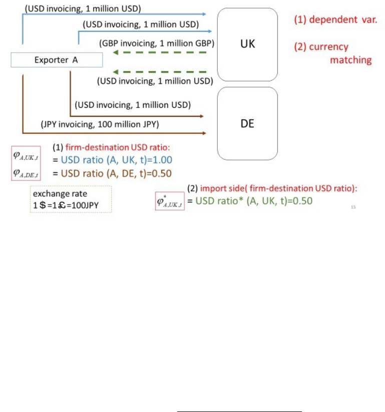
Figure 1: The invoicing currency ratio and currency matching

Note: This ﬁgure represents the subset of transaction-level data in the data and shows how the

calculation of the invoicing currency ratio is structured.

include the identity of the reporting company and the foreign trading partner, product char-

acterization, corresponding HS 9-digit code, the value and quantity of transactions, and the

invoicing currency. The value of each transaction record has ﬁve arguments: invoicing currency

c, ﬁrm i, product j, partner country k, and year t: val(c, i, j, k, t). We construct the dollar

invoicing ratio by exporter-destination pairs in year t as follows.

i,k,t

= IC

c=D,i,k,t

j,c=D

val(c, i, j, k, t)

c,j

val(c, i, j, k, t)

, (4)

where c = D represents the US dollar invoicing currency. The numerator in equation (4)

represents the value of transactions invoiced in US dollars, and the denominator is the value

of all transactions. For the rest of the paper, we use IC with corresponding subscripts, D, to

denote the dollar invoice ratio.

Figure 1 demonstrates how an invoicing currency ratio, ϕ

i,k,t

, is calculated with the example

of four export transactions by exporter A. In the example, export transactions are invoiced in

diﬀerent currencies; however, we set exchange rates so that the values of all transactions are

equivalent in the common currency. Exporter A exported to the UK in two transactions, both

invoiced in US dollars, and to Germany in two transactions, one in US dollars and the other in

Japanese yen. In this case, ϕ

A,UK,t

= 1.00 and ϕ

A,DE,t

= 0.50.

2.3 Determinants of Currency Choice

Gopinath, Boz, Casas, D´ıez, Gourinchas, and Plagborg-Møller (2020) propose the dominant

currency paradigm in which exporters set prices in a dominant currency, face strategic com-

plementarities in pricing, and use foreign inputs. Following their dominant currency paradigm

model, they empirically conﬁrm the model’s implications by using the worldwide coverage of

bilateral trades. The theoretical model in Amiti, Itskhoki, and Konings (2022) showed that

the desired exchange rate pass-through depends on the exposure of the ﬁrm’s marginal cost to

exchange rates, ϕ, and the exposure of the ﬁrm’s desired markup to exchange rates, γ. In turn,

the invoicing currency is chosen based on the lowest variance of the desired price expressed in

that currency. Amiti, Itskhoki, and Konings (2022) proxy for ϕ with the ﬁrm’s share of im-

ported inputs in total variable costs, sourced in foreign (non-euro) currencies for the Belgian

exporters. The proxy variables for γ use the export-weighted average currency use of the ﬁrm’s

Belgian competitors in a given destination industry. Using the UK transaction level of exports

and imports between 2010 and 2016, Crowley, Han, and Son (2021) ﬁnd that the US dollar is

an invoicing currency choice for UK exports to extra-EU destinations, i.e., transactions with all

countries outside of the EU, are driven by strategic complementarities, operational hedging, and

prior experience.

2.3.1 Strategic Complementarity Indices

The ﬁrst strategic complementary index we introduce is the likelihood of dollar use by the

competitors in the destination market, k.

k,t

= IC

c=D,−i,k,t

c=D,−i,j

val(c, i, j, k, t)

c,−i,j

val(c, i, j, k, t)

(5)

where −i indicates that the sum is taken over for all ﬁrms except ﬁrm i.

The second strategic complementary index is the likelihood of dollar use by the competitors

in the industries associated with the ﬁrm. This takes two steps. First, we construct the dollar

invoicing ratio in each HS 4-digit industry.

c=D,−i,j,t

c=D,−i,k

val(c, i, j, k, t)

c,−i,k

val(c, i, j, k, t)

(6)

c=D,−i,j,t

is the dollar ratio in industry j and is adjusted for each Japanese exporter. Then,

Figure 2: Strategic complementarity variables

Note: This ﬁgure represents the subset of transaction-level data in the data and shows how the

calculation of strategic complementarity variables is structured.

we calculate each ﬁrm’s weighted average of these industry indices.

i,t

(j)IC

c=D,−i,j,t

(7)

where p

i,t

(j) is the share of ﬁrm i’s export in HS 4-digit industry j in year t. This index

reﬂects how much dollar invoice is used by the competitors in the industries with which ﬁrm i

is associated.

Figure 2 shows how the strategic complementarity indices are calculated. In this ﬁgure,

all transactions by all exporters are shown. There are three export transactions to the UK

and Germany each. The product categories of these transactions are either HS8701 or HS8705

at the HS 4-digit industry. Exchange rates are set so that the values of all transactions are

equivalent in the common currency. The strategic complementarity index at the country level

is straightforward as in equation (5). Two out of three transactions to the UK are invoiced

in US dollars, so γ

UK,t

= 0.66. Similarly, we can calculate the US dollar invoicing ratio in

Germany; γ

DE,t

= 0.33. The calculation of the strategic complementarity index reﬂecting

industry dimension involves two steps. First, the US dollar invoicing ratios are calculated for

each industry as in equation (6). Only one out of four transactions in HS8701 industry is

invoiced in US dollars; therefore, IC

USD,HS8701,t

= 0.25. Similarly, the US dollar invoicing

ratio for HS8705 is calculated as IC

USD,HS8705,t

= 1.00. Second, these indices are used to

calculate the industry-weighted average for each exporter, as in Equation (7). If ﬁrm A exports

80 percent to the HS8701 industry and 20 percent to the HS8705 industry, the industry-wise

strategic complementarity index for ﬁrm A is γ

A,t

= 0.40.

2.3.2 Currency Matching Index

Amiti, Itskhoki, and Konings (2022) construct the Belgian ﬁrm’s import intensity as the

ratio of total imports from outside the eurozone to total variable costs. They use this variable

as a proxy for the ﬁrm’s marginal cost sensitivity to the exchange rate. The underlying implicit

assumption is that these imports are not invoiced in euros.

If, as an extreme example, all

imports from non-Euro countries are invoiced in euros, the Belgian ﬁrms are unaﬀected by a

change in the exchange rate, at least from the importing side.

Theoretical models of exchange rate pass-through and currency invoicing explicitly consid-

ered the imported inputs in the international ﬁnance literature.

Chung (2016) is one of the

ﬁrst empirical studies that highlighted the link between imported inputs and exporters’ deci-

sions on invoicing currency. Chung (2016) introduced the ratio of imported inputs invoiced in

the exporter’s currency to its total imported inputs at the UK ﬁrm level to consider the role of

exporter’s operational hedging behavior.

Our approach to constructing an import intensity variable is to consider the invoicing cur-

rency choice in imports, similar to (Crowley, Han, and Son 2021). The new contribution of

this study is to introduce three indices that are complementary to each other. The ﬁrst is a

straightforward extension of the currency choice variable to the import side. The dollar used

on the import side is matched with the export side at the ﬁrm-country level. Note that this

variable has two dimensions, in ﬁrms and destinations, whereas the import intensity index in

Amiti, Itskhoki, and Konings (2022) varies only over ﬁrms.

The currency matching variable

A,t

= 0.8 ∗ IC

USD,HS8701,t

+ 0.2 ∗ IC

USD,HS8705,t

= 0.40

Therefore, Amiti, Itskhoki, and Konings (2022) further breaks the import intensity index into euro-invoiced

import intensity and non-euro-invoiced import intensity for alternative speciﬁcations.

The role of imported inputs in exporting ﬁrms has also been well examined in the international trade literature.

Imported inputs can be used to measure the degree of participation in global value chains as surveyed in Johnson

(2018). Imported inputs can be a source of growth engine for multinational ﬁrms (Halpern, Koren, and Szeidl

2015).

Operational hedge is also found essential even in domestic transactions in the dollarization economy of Uruguay

(Licandro and Mello 2019). On the other hand, Lyonnet, Martin, and Mejean (2022) found that large EU ﬁrms

are more willing to use non-euro invoicing if ﬁnancial hedging tools are available.

In fact, the import intensity index in Amiti, Itskhoki, and Konings (2022) is also time-invariant, whereas our

is formulated as the following with an asterisk indicating the importing side:

∗

i,k,t

= IC

∗

c=D,i,k,t

j,c=D

val

∗

(c, i, j, k, t)

c,j

val

∗

(c, i, j, k, t)

(8)

Figure 1 shows that exporter A imports from the UK but not from Germany. In this case, we

can calculate ϕ

∗

A,UK,t

= 0.50, but not for Germany.

In regression models in the following section, We implicitly assume that exporters make an

invoicing currency choice, given the invoicing currency of their imports. However, a priori, there

is no consensus on the causality direction, and we face a simultaneity problem. To address this

endogeneity issue, we introduce the second and the third ratios that are the import side version

of equations (5) and (7).

∗

k,t

= IC

∗

c=D,k,t

c=D,i,j

val

∗

(c, i, j, k, t)

i,j

val

∗

(c, i, j, k, t)

(9)

∗

i,t

∗

i,t

(j)IC

∗

c=D,j,t

(10)

These two indices are the US dollar invoicing ratios of the competitors’ imports, therefore not

directly linked to ﬁrm i’s decision on invoicing currency choice of its exports. We use them as

instrumental variables when we include the import intensity index, i.e., equation (8).

2.3.3 Control variables

The variables of interest in this study are two strategic complementarity variables and the

currency-matching variable we discussed in the previous subsections. In this subsection, we

describe other control variables that capture the other eﬀects on currency choice. We introduce

ﬁrm size and market share variables to control individual ﬁrm characteristics. Devereux, Dong,

and Tomlin (2017) found that market shares of both exporters and importers matter for exchange

rate pass-through.

The ﬁrm size variable is the natural log of the ﬁrm i’s total export to destination k:

lnSize

i,k,t

= ln

c,j

val(c, i, j, k, t). As the robustness check in section 4.3, we use alterna-

tive deﬁnitions for ﬁrm size: total export to all destinations, the sum of export to and import

from country k, and the sum of export to and import from all countries. The ﬁrst of these

alternatives corresponds to the ﬁrm size used in Crowley, Han, and Son (2021).

Market share variable is the value-weighted average of market shares at HS 4-digit indus-

tries: MShare

i,t

(

c,k

val(c, i, j, k, t)/

c,i,k

val(c, i, j, k, t)). For each 4-digit industry

indices change by year.

(across all destination countries) in which ﬁrm i exports, the market share is calculated. Then,

these market shares are taken average with ﬁrm i’s export share at HS 4-digit industries,w

as weights.

In robustness section 4.3, we also use three alternative deﬁnitions for market

share. Two alternatives use HS 2-digit and HS 6-digit levels instead of HS 4-digit level. The

last deﬁnition uses the market share in the destination country.

Fixed eﬀects can potentially be constructed at the level of ﬁrms, destination countries, indus-

tries, and years. We avoided using ﬁrm-ﬁxed eﬀects because the ﬁrm-year-varying market share

variable, MShare

i,t

, already controls this dimension. Similarly, we do not use destination-ﬁxed

eﬀects because the strategic complementarity variable, γ

k,t

, captures destination characteristics.

Industry-ﬁxed eﬀects are not appropriate because the observation unit in this study aggregates

over industries. Therefore, we only include year-ﬁxed eﬀects to control for time-varying eﬀects

on a ﬁrm’s currency choice.

3 Empirical Model of Invoicing Currency Choice

The data records all export and import declarations individually.

Therefore, even within

a year, the same product is exported multiple times to the same destination market by the

same exporter.

Instead of analyzing exports at each declaration, we pooled exports by the

exporter and destination market each year. The advantage of pooling products at this level is

that we can measure the likelihood of choosing a speciﬁc invoicing currency for an exporter in

a particular destination market. Therefore, the choice of invoicing currency is aggregated at

the pair of exporter and destination market as the dollar ratio, ϕ

i,k,t

with subscripts denoting

exporter i, destination country k, and year t, see equation (4). The choice of invoicing currency

is also constructed for imports as ϕ

∗

i,k,t

, see equation (8).

3.1 Invoicing Currency Choice and Strategic Complementarities

The ﬁrst base model only includes ﬁrm size and strategic complementarity variables. The

dependent variable is the ratio of the values invoiced in the US dollar in total export values by

ﬁrm-destination pair, ϕ

i,k,t

Due to these deﬁnitions in the base model, two ﬁrm characteristics variables measure diﬀerent aspects of

exporters. lnSize

i,k,t

measures the total exports to destination market k whereas M Share

i,t

is a weighted

measure of total exports to all destination countries. A priori, these variables should be free of multicollinearity

problem.

Low-value cargoes under the simpliﬁed customs clearance are excluded from the database.

For example, in the ﬁrst six months of 2014, for about four percent of the sample, diﬀerent invoice currencies

are chosen for the same HS 9-digit export to the same destination country by the same exporter within a month.

i,k,t

= α + β

lnSize

i,k,t

+ β

MShare

i,t

+ β

k,t

+ β

i,t

+ ϵ

i,k,t

(11)

The ﬁrm’s size, lnSize

i,k,t

, is the natural log of the ﬁrm i’s total export to destination k,

the market share of the ﬁrm, MShare

i,t

, is the value-weighted average of market shares at HS

4-digit industries, and the two complementarity indices are the likelihood of dollar invoice in the

destination market, γ

k,t

, and the likelihood of dollar invoice in associated industries, γ

i,t

. The

deﬁnitions of complementarity indices are shown in equations (5) and (7).

The dependent variable is fractional, 0 ≤ ϕ

i,k,t

≤ 1, with non-zero mass at the two extreme

values. The predicted values from an OLS regression cannot be guaranteed to lie between 0 and

1. Therefore, similar to binary dependent variable models, we assume that

E(ϕ

i,k,t

| X

i,k,t

) = G(X

i,k,t

B) (12)

where X

i,k,t

denotes the vector of explanatory variables, B is the vector of parameters, and

G(·) is the standard normal cumulative density function, satisfying 0 < G(z) < 1 for all z ∈ ℜ.

In particular, we apply the fractional response regression proposed by Papke and Wooldridge

(1996).

The expected signs of two strategic complementary indices, γ

k,t

and γ

i,t

, are positive. The

expected sign of ﬁrm size is less evident in the previous studies. Firm size positively correlates

with non-euro invoicing for the Belgian exporters in Table 2 of Amiti, Itskhoki, and Konings

(2022). This non-euro currency includes US dollars, destination currency, and other currencies.

Table 4 of Amiti, Itskhoki, and Konings (2022) further shows that ﬁrm size negatively correlates

with US dollar invoicing. On the other hand, the dollar invoicing by UK exporters is positively

correlated with ﬁrm size in Crowley, Han, and Son (2021). These analyses are based on the

extra-EU exports for Belgian and UK ﬁrms. A signiﬁcant number of observations are excluded

from the original sample. On the market share, the expected sign is ever less clear in previous

empirical evidence. The market share is estimated to positively aﬀect non-euro invoicing for

the Belgian ﬁrms in Amiti, Itskhoki, and Konings (2022); however, the statistical signiﬁcance of

market share disappears when the ﬁrm size variable is introduced in the regression model.

3.2 Currency Matching

Our approach slightly diﬀers from Amiti, Itskhoki, and Konings (2022) and Crowley, Han,

and Son (2021) in implementing the import side variables. Amiti, Itskhoki, and Konings (2022)

use ﬁrm-speciﬁc import intensity, i.e., the ratio of total extra-EU import to total variable costs.

This import intensity is also constructed for non-euro invoicing and dollar invoicing. Construct-

ing this variable requires matching trade data and accounting data by identifying each ﬁrm

in both data sets and is much more data-demanding. However, their index is the average of

the entire sample period and is time-invariant and destination-invariant. Crowley, Han, and

Son (2021), on the other hand, rely solely on the trade data set; therefore, their construction

of import-side indices is similar to ours. Their index is the share of the ﬁrm’s dollar invoiced

imports in its total imports. This variable is time-varying but not destination-varying. Our

index, ϕ

∗

i,k,t

, in equation (8) is both destination-varying and time-varying. This new index has

an important implication when we focus on two-way exporters. More precisely, we deﬁne a

ﬁrm-destination pair as two-way if we observe export and import data in the same year. Note

that the deﬁnition of two-way exporter applies to the pair of ﬁrm-destination so that a ﬁrm can

be two-way for one market and not for another. Our regression model for evaluating a ﬁrm’s

incentive to match the invoice currencies of exports and imports is the following.

i,k,t

= α + β

lnSize

i,k,t

+ β

MShare

i,t

+ β

k,t

+ β

i,t

+ β

∗

i,k,t

+ ϵ

i,k,t

(13)

The analysis with the import-side variables has one drawback: The invoicing currency choice

on exports and imports are simultaneous decisions. Also, from the perspective of the importing

side, a similar relationship between the ﬁrm’s import invoicing and competitors’ import invoicing

should hold.

Alternatively, using γ

∗

k,t

and γ

∗

i,t

as instruments, we also estimate equation (13)

by instrumental variable (IV) fractional probit.

3.2.1 Two-way Exporters

For broad two-way exporters, imports from other countries should aﬀect the invoicing cur-

rency choice of exports. For example, a Japanese exporter exporting to China and importing

from Germany and the US would not be a narrow two-way because it does not import from

the country of export destination, China. The observation of this exporter’s export to China

would be dropped from the above regression when we restrict the sample to narrow two-way

exporters. However, up to the degree of US dollar invoicing for its imports from Germany and

the US, the exporter considers the use of US dollar invoicing for its exports to China. This

concept is adopted by Amiti, Itskhoki, and Konings (2022), and we deﬁne it as broad two-way.

We also estimate equation (13) with the sample of broad two-way exporters, and import side

index, ϕ

∗

i,k,t

, is replaced by ϕ

∗

i,t

, the US dollar ratio for import invoicing at the ﬁrm level.

We estimated an import-side regression analogous to equation (11) and obtained similar results.

Table 2: Invoice currency by exporter type (2014-2020)

all exporters broad two-way narrow two-way

(no. of pairs) 3,043,901 1,949,043 921,088

(no. of ﬁrms) 747,353 187,354 131,923

(trillion yen) 551.9 538.0 495.1

USD 0.51 0.52 0.53

- excl. US (0.35) (0.35) (0.35)

JPY 0.36 0.35 0.34

EUR 0.06 0.07 0.07

LC 0.27 0.28 0.30

- excl. US (0.11) (0.11) (0.11)

Note: Broad two-way exporters are those exporters that also import in the same year. Narrow

two-way exporters are deﬁned over the exporter and destination country pairs that also import

from the same destination country in the same year. These deﬁnitions are applied to the

observations of each year. The ﬁrst row represents the number of exporter-country pairs whereas

the second row indicates the number of distinct exporters. The ratio in parenthesis excludes the

US from the calculation. LC is local currency invoicing.

Table 2 summarizes the use of invoicing currencies by exporter types. The ﬁrst column

represents all exporters, corresponding to the ﬁrst row of Table 1. In the second and third

columns, the summary statistics for invoicing currencies for broadly deﬁned and narrowly deﬁned

two-way exporters are shown, respectively. There are some salient features. Based on our

deﬁnitions of ﬁrm-destination, the number of observations for seven years decreases to about

two-thirds in the broad two-way sample and one-third in the narrow two-way sample. The

corresponding ﬁrms are 747, 187, and 131 thousand ﬁrms for all, broad two-way, and narrow

two-way exporters, respectively. This implies that about 75 percent of Japanese exporters do

not import at all and that about 70 percent of ﬁrms engaging in both exports and imports,

in fact, use (at least) one particular country for both exports and imports. More importantly,

these two-way exporters conduct a large share of exports (in terms of values): 97 percent by

broad two-way and 90 percent by narrow two-way exporters. On the other hand, only a little

diﬀerence exists in the use of invoicing currencies among exporter types.

4 The Empirical Results

For the empirical investigation on the choice of invoicing currency in Japanese exports, we

use the general export and import declarations submitted to Japan Customs, the Ministry of

Finance, between 2014 and 2020. As described in section 3, we use the US dollar invoicing

ratio at the ﬁrm-country level as the dependent variable in the base model and estimate the

regression models (11) and (13). The appendix table A.1 provides the statistical summary of

variables used in the regression models.

4.1 US dollar Invoicing, Dominant Currency

Table 3 shows regression (11) estimation results by all exporters, broadly deﬁned two-way

exporters, and narrowly deﬁned two-way exporters for the panel between 2014 and 2020. The

models are estimated by fractional probit, and the table shows the marginal eﬀects of covari-

ates. The sign of γ

, the US dollar invoicing ratio in the destination k, is positive and it captures

strategic complementarity among exporting ﬁrms. By comparing the magnitude, it is interesting

to ﬁnd that two-way exporters in columns (2) and (3) are more inclined to follow the currency

choice of competitors than the entire sample of exporters in column (1). More speciﬁcally, the

eﬀect of strategic complementarity in the destination country dimension is more substantial for

narrowly deﬁned two-way exporters. Exporters that export to and import from the same country

pay more attention to the competitors’ choice of invoicing currency in that market. Similarly,

the competitors’ currency choice in the corresponding industries, γ

, the weighted average of the

dollar ratio with the ﬁrm’s exporting value by industries as weights, are positive and statistically

signiﬁcant. An exporter is likely to increase the use of US dollars as invoicing currency if the dol-

lar is predominantly used in a destination country and/or in the ﬁrm’s associated industries. On

the other hand, big exporters, measured as large total exports to the corresponding destination

countries or higher market share, lower the use of the US dollar. At this moment, it should not

be confused with the notion implicitly indicating that they prefer the Japanese yen as invoicing

currency. Local currency or other vehicle currency is also possible besides the Japanese yen as

an alternative invoicing currency. We will come back to this issue in subsection 4.2.

Table 3: US dollar invoicing and strategical complementarity, 2014-2020

(1) USD (2) USD (3) USD

Fractional Probit Fractional Probit Fractional Probit

lnSize

i,k,t

-0.0061*** -0.0084*** -0.0096***

(0.0012) (0.0006) (0.0009)

MShare

i,t

(HS4) -0.9715*** -1.0216*** -0.7431***

(0.1349) (0.1380) (0.1876)

k,t

(SC Country USD) 0.2573*** 0.3442*** 0.4528***

(0.0213) (0.0132) (0.0113)

i,t

(SC HS4 USD) 1.1298*** 1.1140*** 1.0982***

(0.0187) (0.0116) (0.0147)

year ﬁxed eﬀects yes yes yes

N. of observations 3,043,872 1,949,018 921,088

Psuedo R

0.35 0.27 0.29

ﬁrm-type all broad two-way narrow two-way

Note: The dependent variable is the US dollar invoicing currency ratio. The coeﬃcients and

standard errors estimated by a fractional probit model are shown for the marginal eﬀect. The

standard errors in parenthesis are clustered by the import size of destination countries and years.

broad two-way exporters are those exporters that also import in the same year. Narrow two-

way exporters are deﬁned over the exporter and destination country pairs that also import from

the same destination country in the same year. ***, **, * represent one, ﬁve, and ten percent

signiﬁcance level.

Table 4: US dollar invoicing with import side invoicing currency, 2014-2020

(1) USD (2) USD (3) USD (4) USD (5) USD w/o US

Fractional Probit IV Frac. Probit Fractional Probit Frational Probit IV Frac. Probit

lnSize

i,k,t

-0.0074*** -0.0073*** -0.0082*** -0.0077*** -0.0082***

(0.0008) (0.0007) (0.0008) (0.0006) (0.0004)

MShare

i,t

(HS4) -0.7316*** -0.7317*** -0.6870*** -0.9607*** -0.6207***

(0.1709) (0.1708) (0.1724) (0.1302) (0.1448)

k,t

(SC Country USD) 0.2676*** 0.2651*** 0.4248*** 0.3359*** 0.1857***

(0.0127) (0.0168) (0.0115) (0.0131) (0.0119)

i,t

(SC HS4 USD) 0.9664*** 0.9647*** 1.0002*** 1.0517*** 0.8893***

(0.0164) (0.0211) (0.0187) (0.0129) (0.0207)

∗

i,k,t

(USDRatio im) 0.1925*** 0.1954*** 0.2136***

(0.0056) (0.0135) (0.0132)

∗

i,t

(byﬁrm USDRatio im) 0.1203*** 0.0827***

(0.0079) (0.0038)

year ﬁxed eﬀects yes yes yes yes yes

N. of observations 921,088 921,088 921,088 1,949,018 809,308

Pseudo R

0.33 0.30 0.27

ﬁrm-type narrow two narrow two narrow two broad two narrow two

Note: The dependent variable is the US dollar invoicing currency ratio. The coeﬃcients and standard errors are shown for

marginal eﬀect. The standard errors in parenthesis are clustered by the import size of destination countries and years. broad

two-way exporters are those exporters that also import in the same year. Narrow two-way exporters are deﬁned over the exporter

and destination country pairs that also import from the same destination country in the same year. ***, **, * represent one,

ﬁve, and ten percent signiﬁcance level.

Table 3 shows that the results of two-way exporters are qualitatively the same as those

of all exporters, including one-way exporters. Table 4 presents the estimated results with the

dollar invoicing ratio on the import side. This variable is not introduced here to relate the

exporter’s choice of invoicing currency with the competitors’ currency strategies as in Table

3. This analysis examines a possible incentive for ﬁrms to match currencies on the asset, i.e.,

receipt from exports, and debit side, i.e., payment for imports, of the balance sheet, and we call

it a currency-matching incentive. If the cash inﬂow from exports and cash outﬂow for imports

are in the same currency, the exchange rate risk hinges only on the net balance.

The ﬁrst column in Table 4 includes the US dollar ratio of imports, ϕ

∗

i,k,t

, as an additional

explanatory variable for narrow two-way exporters. The US dollar ratio for imports is similarly

constructed as the US dollar ratio, the dependent variable, for the same ﬁrm and the same

country. The US dollar ratio for imports is statistically signiﬁcant. The estimated coeﬃcient

indicates that a ten-percentage point increase in the US dollar ratio for imports in the same

industry and country induces a 1.93 percentage point increase in the dollar use in exports.

The endogeneity issue may exist for the import-side variable.

In the second column, we re-

estimated the model as in column (1) but used γ

∗

and γ

∗

as instruments in the instrumental

variable fractional probit model. The estimated results are similar to those in column (1).

In columns (3) and (4), we replace the US dollar ratio for ﬁrm-destination import,ϕ

∗

i,k,t

, with

the US dollar ratio for ﬁrm import, ϕ

∗

i,t

, which is not destination-speciﬁc. Firm size, market

share, and strategic complementarity variables are only marginally aﬀected, and their estimates

remain statistically signiﬁcant at the one percent level. In column (3), the magnitude of the

currency-matching coeﬃcient at the ﬁrm level is smaller than the currency-matching variable

at the ﬁrm-destination level in column (1). This result implies that a typical ﬁrm pays more

attention to balancing the currency ﬂows on a country basis than managing every currency

ﬂow over the ﬁrm’s entire accounting. Column (4) shows that the US dollar invoicing ratio

for broad two-way exporters is less sensitive to the ﬁrms’ US dollar invoicing for imports. To

summarize, narrow two-way exporters are more inclined than broad two-way exporters to match

the invoicing currency of exports to the overall invoicing currency of imports, and they pay more

attention to a country basis for currency matching.

We estimated the corresponding estimation model as of equation (11) for imports and found that similar

results hold for the import side.

4.2 Vehicle Currency, Producer Currency, and Local Currency Invoicing

We found supporting evidence for strategic complementarities and currency matching for

the US dollar invoicing in the preceding section. In this section, we investigate other currency

invoicing practices and show that the central message holds.

Table 5: Producer currency pricing and local currency pricing

(1) JPY (2) JPY (3) LC (4) LC

Frac. Probit IV Frac. Probit Frac. Probit IV Frac. Probit

lnSize

i,k,t

0.0046*** 0.0017*** 0.0024*** 0.0033***

(0.0006) (0.0005) (0.0004) (0.0005)

MShare

i,t

(HS4) 0.1242 0.2521*** -0.9528*** -0.7118***

(0.0996) (0.0904) (0.1116) (0.1042)

k,t

(SC Country JPY(LC)) 0.3811*** 0.2806*** 0.3797*** 0.2560***

(0.0258) (0.0193) (0.0069) (0.0267)

i,t

(SC HS4 JPY(LC)) 1.0501*** 0.9623*** 0.7737*** 0.7137***

(0.0063) (0.0076) (0.0311) (0.0379)

∗

i,k,t

(JPY(LC)Ratio im) 0.2168*** 0.1239***

(0.0067) (0.0299)

year ﬁxed eﬀects yes yes yes yes

N. of observations 921,088 921,088 921,088 921,088

Psuedo R

0.30 0.41

ﬁrm-type narrow two narrow two narrow two narrow two

Note: The dependent variable is the Japanese yen invoicing ratio in columns (1) and (2) and the local

currency invoicing ratio in columns (3) and (4). The coeﬃcients and standard errors are shown for the

marginal eﬀect. Standard errors in parenthesis are clustered by the import size of destination countries

and years. Narrow two-way exporters are deﬁned over the pairs of exporter and destination country that

also import from the same destination country in the same year. ***, **, * represent one, ﬁve, and ten

percent signiﬁcance level.

4.2.1 Vehicle Currency: The US dollar Invoicing to non-US markets

Including the US as a destination country in the estimation for the US dollar invoicing may

bias the estimates. The US dollar invoicing to non-US destination countries is a form of vehicle

currency invoicing. This pervasive use of the US dollar in trade with countries other than the

U.S. supports the fundamental idea of the dominant currency paradigm in the literature, for

example, in Gopinath, Boz, Casas, D´ıez, Gourinchas, and Plagborg-Møller (2020). Therefore,

we re-estimate the regressions, excluding the US as the destination country.

Column (5) in Table 4 presents the estimated equation (13) results by excluding the US from

destination countries. This robustness check conﬁrms that the qualitative results remain intact

even when the US is excluded from the sample, reducing approximately 12 percent of ﬁrm-

destination observations. The impact of strategic complementarity in the destination market is

lower, consistent with our expectations. In the competing industries, it is also lower but less

substantially. The eﬀect of currency matching is slightly more signiﬁcant. To summarize, the

preceding results of US dollar invoicing do not hinge on the presence of the US in the sample,

but vehicle currency use or the dominant currency role of the US dollar is supported in samples

other than the United States.

4.2.2 Producer Currency Invoicing: Japanese yen Invoicing

Examining whether the strategic complementarity and currency matching mechanisms also

work on other invoicing currencies is important. In our data set, we turn to the producer

currency invoicing, i.e., the Japanese yen invoicing. The dependent variable is the Japanese yen

invoicing ratio at the ﬁrm-destination pairs. The explanatory variables are similarly constructed

for the Japanese yen invoicing. The ﬁrst two columns of Table 5 present the estimation results

for the Japanese yen invoicing.

There is one noteworthy diﬀerence between the US dollar and Japanese yen invoicing. The

estimated signs of size and market share variables are opposite of the US dollar invoicing model.

Therefore, it implies that a larger-sized Japanese exporter is more likely to choose the Japanese

yen over the US dollar. The market share, representing the competitiveness of exporters, allows

the Japanese exporters to use their own currency. This is consistent with the results found in Ito,

Koibuchi, Sato, and Shimizu (2012) that ﬁrms that responded positively to the questionnaire

about their international competitiveness are more likely to choose Japanese yen invoicing.

Besides these diﬀerences, the qualitative results are the same for the US dollar and Japanese

yen invoicing.

4.2.3 Local Currency Invoicing

Columns (3) and (4) in Table 5 show the results for local currency pricing. The estimated

sign of the size variable is positive and opposite of the US dollar invoicing model. In contrast,

the market share variable shows the same sign as in the US dollar invoicing model. The size

variable is consistent with the result in Amiti, Itskhoki, and Konings (2022) with the subsample

analysis of dollar-invoicing against local-currency invoicing for non-US and non-USD-pegging

countries. The estimated coeﬃcients of the ﬁrm’s employees are negative and statistically sig-

niﬁcant, implying a larger ﬁrm is more likely to invoice in local currencies.

Regarding strategic complementarity and currency matching variables, the estimates are a

little smaller than the US dollar invoicing, but they are all statistically signiﬁcant at the one

percent level. Therefore, regardless of the dominant vehicle, producer, or local currency, strategic

complementarity and currency-matching mechanisms for choosing the invoicing currency work

for Japanese exporters.

4.3 Robustness: Alternative size, market share, and strategic complemen-

tarity

Some of the control variables used so far can be deﬁned diﬀerently. In this section, we re-

estimate the models by replacing the original variables with alternatives. The estimated results

of the base model, column (2) in Table 4, are reproduced in column (1) of Table 6. First, we

evaluate the robustness of ﬁrm size. The size of ﬁrms is measured initially as export values by a

ﬁrm to a destination country. Alternatively, export values by a ﬁrm to all destination countries

in column (2), the sum of export and import values by a ﬁrm to a destination country in column

(3), and the sum of all exports and imports by a ﬁrm in column (4) are used in the model. The

estimated coeﬃcients of alternative size variables are consistent with the estimate in column

(1); they are negative and statistically signiﬁcant at the one percent level, and the estimates are

smaller.

Second, we check the robustness of market share. Alternative variables are deﬁned as the

ﬁrm’s export value to total export values by all Japanese exporters in a destination country

in column (5), and HS 2-digit and 6-digit instead of HS 4-digit level are used in columns (6)

and (7), respectively. All the estimates are consistent with the result of the base model. The

magnitude varies among alternatives due to decreased measure of market share as industry

classiﬁcation becomes broader. Third, the strategic complementarity variable is replaced with

those with diﬀerent levels of industry classiﬁcation in columns (8) and (9). The estimated results

are almost identical to the result of the original variable. In summary, the results in previous

sections are robust to alternative deﬁnitions of explanatory variables.

See, Table IV in Amiti, Itskhoki, and Konings (2022).

Table 6: Alternative deﬁnitions of size, market share, and strategic complementarity

(1) (2) (3) (4) (5) (6) (7) (8) (9)

alternative variable size (e, all) size (e&i) size (e&i, all) ms (dest.) ms (HS2) ms (HS6) sc (HS2) sc (HS6)

size -0.0073*** -0.0064*** -0.0044*** -0.0035*** -0.0075*** -0.0072*** -0.0074*** -0.0075*** -0.0074***

(0.0007) (0.0007) (0.0008) (0.0007) (0.0007) (0.0007) (0.0007) (0.0007) (0.0007)

ms -0.7317*** -0.5842*** -0.9623*** -0.8997*** -0.0847* -2.6846*** -0.2910*** -0.3568*** -0.7524***

(0.1708) (0.1678) (0.1736) (0.1784) (0.0515) (0.2497) (0.0820) (0.1188) (0.1733)

k,t

(SC country) 0.2651*** 0.2469*** 0.2529*** 0.2462*** 0.2661*** 0.2645*** 0.2654*** 0.2482*** 0.2585***

(0.0168) (0.0189) (0.0180) (0.0194) (0.0168) (0.0168) (0.0168) (0.0172) (0.0169)

i,t

(SC industry) 0.9647*** 0.9835*** 0.9552*** 0.9647*** 0.9624*** 0.9661*** 0.9637*** 1.0000*** 0.9404***

(0.0211) (0.0202) (0.0208) (0.0198) (0.0213) (0.0213) (0.0211) (0.0197) (0.0214)

∗

i,k,t

(USDRatio im) 0.1954*** 0.1890*** 0.2096*** 0.2044*** 0.1952*** 0.1953*** 0.1955*** 0.2053*** 0.2067***

(0.0135) (0.0143) (0.0135) (0.0136) (0.0135) (0.0136) (0.0135) (0.0142) (0.0135)

year ﬁxed eﬀects yes yes yes yes yes yes yes yes yes

NOB 921,088 921,088 921,088 921,088 921,088 921,088 921,088 921,088 921,088

N. of ﬁrms 131,923 131,923 131,923 131,923 131,923 131,923 131,923 131,923 131,923

Note: The dependent variable is the US dollar invoicing currency ratio. These models are estimated by instrumental variable fractional

probit, and the coeﬃcients are marginal eﬀects. Standard errors in parenthesis are clustered by the import size of the destination country

and years. Firm types are narrow two-way exporters. ***, **, * represent one, ﬁve, and ten percent signiﬁcance level. The ﬁrst column

is the base model and corresponds to column (2) in Table 4. From columns (2) to (4), alternative deﬁnitions for ﬁrm size are used; (e,

all) export values to all destination countries, (e&i) the sum of export and import values to the same destination country, and (e&i, all)

the sum of export and import values to and from all countries. From column (5) to (7), alternative deﬁnitions for market share are used:

(dest.) market share of ﬁrms’ export values in the destination country, (HS2) market share of ﬁrms’ export in the corresponding HS 2-digit

categories, and (HS6) market share of ﬁrms’ export in the corresponding HS 2-digit categories. In the last two columns, alternative strategies

complementarity variables are constructed at the level of HS 2-digit and 6-digit industries.

5 New Exporters

As discussed in section 3.2, one way to address the simultaneous problem of choosing in-

voicing currency in exports and imports is to use instrumental variable estimation or two-stage

least squares. These are statistical methods to obtain consistent estimators. We applied the

instrumental variable fractional probit estimation method in the previous section. Alternatively,

we propose to focus on the subsample of ﬁrms that have yet to record international trade trans-

actions in the last year. Therefore, the invoicing currency decision we analyze here is the ﬁrst

decision on new exporters’ invoicing currency. In this way, we can at least exclude the pre-

determined decision of the previous year on imports from aﬀecting the current year’s decisions

on exports. For these subgroups of ﬁrms, we re-estimate the regression model in equation (13).

In the following years, ﬁrms may reevaluate the ﬁrst decision and may alter the invoicing cur-

rency. This analysis implies that a currency-matching mechanism gradually forms as a ﬁrm

accumulates years of trade experience

The ﬁrst column in Table 7 shows the estimation results of equation (13) for 2015, including

all narrow two-way exporters. Even for this particular single year, we conﬁrm that strategic

complementarity variables and currency matching variables, at the ﬁrm-destination level, sig-

niﬁcantly impact the invoice decision of the Japanese exporters. Size eﬀect and market share

eﬀects are also consistent with the panel results.

Crowley, Han, and Son (2021) also examine the dynamic eﬀects of dollar invoicing for UK ﬁrms. However,

their focus is on the impact of the experience of using the dollar in any markets on choosing the dollar invoice in

a new market.

Table 7: New Exporters in 2015

previous year no trade no trade

lnSize

i,k

-0.0099*** -0.0199*** -0.0112*** -0.0207***

(0.0012) (0.0015) (0.0014) (0.0016)

MShare

(HS4) -1.0604*** 0.0615 -0.9712*** 0.0473

(0.2738) (0.5655) (0.2896) (0.6070)

(SC Country USD) 0.2579*** 0.2009*** 0.4521*** 0.2737***

(0.0497) (0.0305) (0.0305) (0.0270)

(SC HS4 USD) 0.8995*** 1.4673*** 0.9420*** 1.4688***

(0.0512) (0.1226) (0.0419) (0.1278)

∗

i,k

USDRatio im 0.2320*** 0.1698***

(0.0328) (0.0242)

∗

byﬁrm USDRatio im 0.1347*** 0.1328***

(0.0168) (0.0213)

NOB 131,417 5,343 131,417 5,343

N. of ﬁrms 49,935 4,494 49,935 4,494

Note: The dependent variable is the US dollar invoicing currency ratio. These models are

estimated by instrumental variable fractional probit, and the coeﬃcients are marginal eﬀects.

Standard errors in parenthesis are clustered by the import size of the destination country and

years. Firm types are narrow two-way exporters. ***, **, * represent one, ﬁve, and ten percent

signiﬁcance level.

Figure 3: The eﬀects of currency matching on new exporters

Note: The marginal eﬀects are estimated by instrumental variable fractional probit. The

vertical lines represent the conﬁdence interval of two standard deviations for the impact of

currency matching on the choice of invoicing currency in ﬁrm-destination pairs. All four panels

are based on the estimated results for narrowly deﬁned two-way exporters. For the deﬁnitions

of currency matching, the upper panels use the ﬁrm-destination invoicing currency ratio,

whereas the lower panels use the ﬁrm-level invoicing currency ratio. The left panels show the

results without restrictions on the previous year’s experience. The right panels show the

sample with no trade in the last year.

The second column limited the sample to only new exporters in 2015. More precisely, the

sample included only narrow two-way exporters in 2015, but these exporters did not export to

or import from any countries in 2014. Regarding the number of ﬁrm-destination observations,

compared with column (1), new exporters were about four percent of all exporters in 2015.

Regarding the number of ﬁrms, new exporters in 2015 were about ten percent of all exporters.

By replacing the currency matching variable with the ﬁrm-level measure, the third and fourth

columns show the estimation results of equation (13) for all exporters and new exporters, re-

spectively. In columns (2) and (4), the estimated coeﬃcients remain statistically signiﬁcant for

ﬁrm size and two strategic complementarity indices. On the other hand, the market share is not

statistically signiﬁcant. The variable of interest in this section is currency matching variables,

∗

i,k,t

in column (2) and ϕ

∗

i,t

in column (4). The noteworthy point is that the magnitude of the

estimate for the US dollar invoicing ratio substantially declined for new exporters, although still

statistically signiﬁcant.

The eﬀects of currency matching for new exporters for other years are summarized in Figure

The ﬁgure shows the point estimate and two standard deviation bands for the currency-

matching variable. The estimates of currency matching variables at the ﬁrm-destination level

are shown in the upper panel, and those of ﬁrm-level currency matching are shown in the lower

panel. The currency matching variables are statistically signiﬁcant at the one percent level when

the sample includes all two-way exporters. However, the eﬀects of currency matching became no

longer statistically signiﬁcant for 2016, 2018, and 2020 at the two standard deviations level when

the sample only included new exporters. There are some diﬀerences in the estimation results

among sample years; however, the qualitative results remain the same, namely, that currency

matching evidence is weak at best for new exporters.

We have shown in the previous section that exporters choose their invoicing currency based

on strategic complementarity and currency matching. This mechanism holds for the US dollar

invoicing as well as producer currency invoicing, i.e., the Japanese yen invoicing in this study and

local currency pricing. New exporters also choose their invoicing currency based on imitating

their competitors’ decisions in the destination country and the competing industries. However,

currency matching is not the primary force for new exporters. How can this result of new

exporters reconcile with the result of experienced exporters who consider currency matching as

an essential factor for invoicing currency decisions?

One interpretation of these results is the following. A new exporter enters a destination

market and observes what other competitors are doing, including invoicing currency choices.

The estimates of all variables are shown in the appendix tables.

Exporters do not directly observe their competitors’ invoicing currency, but they face business practices and

An exporter may import intermediate inputs from the same country but accept the import

contract with the speciﬁed invoicing currency. As an exporter continues these transactions for

several years, currency matching becomes an important issue. It may renegotiate with the

incumbent trade partner about altering the invoicing currency or switch to a new partner that

accepts the invoicing currency of the exporter’s choice.

6 Discussions and Conclusions

We contribute to the literature by providing evidence of the Japanese exporters, not only

as another example but as a country not using the US dollar or euro as its own currency nor

being involved in dominant currency regimes, such as the UK or Canada. No study using this

new database has appeared because the data set became available only in 2022. This is not to

claim that no previous studies examined the invoicing currency choice of Japanese exporters.

Ito, Koibuchi, Sato, and Shimizu (2012) and Ito, Koibuchi, Sato, and Shimizu (2018) conducted

multi-year questionnaire surveys to the listed multinational corporations in Japan and concluded

that foreign exchange risk management is the driving force for the dominating share of US dollar

invoicing for Japanese exporters, especially to the US and China as destination markets. They

also found that intra-ﬁrm trade occupies a lion’s share of international trade for multinational

ﬁrms, and the parent ﬁrms headquartered in Japan tend to use the currency of subsidiaries’

locations. This study complements the earlier ﬁndings that the competitors’ currency choice

and matching with the invoicing currency of imports are also important factors for invoicing

currency choice for Japanese exporters.

In addition, we focus our attention on two-way exporters and provide narrow and broad

deﬁnitions. A broader deﬁnition of two-way exporters includes a ﬁrm that imports from country

A and exports to country B. As long as a ﬁrm experiences exports and imports in the same year

regardless of which countries, by a broader deﬁnition, it is labeled as a broad two-way exporter.

Our deﬁnition of narrow two-way exporter excludes those ﬁrms.

This narrow deﬁnition has

important implications. Firms surviving this screening may be more active in intra-ﬁrm trade,

especially if located in the middle of a vertical production network. Another plausible scenario

is that the sample merely captures the fact that narrow two-way exporters are trading with big

countries with a prominent share in both producing and consuming in the world, such as the

standards for pricing when they enter the market. Their trade counterparts will likely request new exporters to

follow the current business practices.

More precisely, our deﬁnition does not mechanically exclude a ﬁrm that imports from A and exports to B. It

is labeled a two-way exporter as long as it also imports from B.

United States. We conﬁrmed that the latter is not a decisive factor, as shown by the analysis

of excluding the US from the sample in section 4.2.1. More importantly, we ﬁnd evidence of

matching with invoicing currency of imports, ϕ

∗

i,k

, even when we restrict to this narrow deﬁnition

of two-way exporters, which should make detecting the eﬀect more diﬃcult.

For future research, this study suggests an essential extension to the exchange rate pass-

through (ERPT) literature for Japanese ﬁrms. Gopinath, Itskhoki, and Rigobon (2010) in-

vestigate how currency choice is endogenously chosen and aﬀects the observed exchange rate

pass-through. The US import price survey data collected by the BLS are examined for the

invoicing currency for their study. The ERPT regressions are estimated for US imports, distin-

guishing those invoiced in the US dollar and those invoiced in non-US dollar currencies. They

ﬁnd that ERPT for goods invoiced in US dollars is about 25 percent, and ERPT for non-US dol-

lars is about 95 percent. The Devereux, Dong, and Tomlin (2017) study utilizes transaction-level

data on Canadian import. Most Canadian imports are invoiced in US dollars because Canada

shares its border with the US and has a solid economic tie to the US. Using the transaction-level

customs data for Canadian imports in monthly frequency between 2002 and 2008, Devereux,

Dong, and Tomlin (2017) found the invoicing currency matters for the observed exchange rate

pass-through. Using Japan Customs data, examining the eﬀect of invoicing currency on the

ERPT is left for our future work.

References

Amiti, M., O. Itskhoki, and J. Konings (2019): “International Shocks, Variable Markups,

and Domestic Prices,” The Review of Economic Studies, 86(6), 2356–2402.

(2022): “Dominant Currencies: How Firms Choose Currency Invoicing and Why it

Matters,” The Quarterly Journal of Economics, 137(3), 1435–1493.

Boz, E., C. Casas, G. Georgiadis, G. Gopinath, H. Le Mezo, A. Mehl, and T. Nguyen

(2022): “Patterns of invoicing currency in global trade: New evidence,” Journal of Interna-

tional Economics, 136, 103604.

Chung, W. (2016): “Imported inputs and invoicing currency choice: Theory and evidence from

UK transaction data,” Journal of International Economics, 99, 237–250.

Corsetti, G., M. Crowley, and L. Han (2022): “Invoicing and the dynamics of pricing-to-

market: Evidence from UK export prices around the Brexit referendum,” Journal of Inter-

national Economics, 135, 103570.

Crowley, M., L. Han, and M. Son (2021): “Dominant currency dynamics: Evidence on

dollar-invoicing from UK exporters,” .

Devereux, M. B., W. Dong, and B. Tomlin (2017): “Importers and exporters in exchange

rate pass-through and currency invoicing,” Journal of International Economics, 105, 187–204.

Gopinath, G., E. Boz, C. Casas, F. J. D

ıez, P.-O. Gourinchas, and M. Plagborg-

Møller (2020): “Dominant Currency Paradigm,” American Economic Review, 110(3), 677–

719.

Gopinath, G., O. Itskhoki, and R. Rigobon (2010): “Currency Choice and Exchange Rate

Pass-Through,” American Economic Review, 100(1), 304–336.

Gopinath, G., and R. Rigobon (2008): “Sticky Borders,” The Quarterly Journal of Eco-

nomics, 123(2), 531–575.

Halpern, L., M. Koren, and A. Szeidl (2015): “Imported Inputs and Productivity,” Amer-

ican Economic Review, 105(12), 3660–3703.

Ito, T., S. Koibuchi, K. Sato, and J. Shimizu (2012): “THE CHOICE OF AN INVOIC-

ING CURRENCY BY GLOBALLY OPERATING FIRMS: A FIRM-LEVEL ANALYSIS OF

JAPANESE EXPORTERS,” International Journal of Finance & Economics, 17(4), 305–320.

(2018): Managing Currency Risk: How Japanese Firms Choose Invoicing Currency.

Edward Elgar.

Johnson, R. C. (2018): “Measuring Global Value Chains,” Annual Review of Economics,

10(1), 207–236.

Licandro, G., and M. Mello (2019): “Foreign currency invoicing of domestic transactions

as a hedging strategy: evidence for Uruguay,” Journal of Applied Economics, 22(1), 622–634.

Lyonnet, V., J. Martin, and I. Mejean (2022): “Invoicing Currency and Financial Hedg-

ing,” Journal of Money, Credit and Banking, 54(8), 2411–2444.

Papke, L. E., and J. M. Wooldridge (1996): “Econometric methods for fractional response

variables with an application to 401(k) plan participation rates,” Journal of Applied Econo-

metrics, 11(6), 619–632.

A Appendix:

The list of 21 Asian countries included in Table 1

Bangladesh, Bhutan, Brunei, Cambodia, India, Indonesia, Republic of Korea, Laos, Malaysia,

Maldives, Mongolia, Myanmar, Nepal, Pakistan, Philippines, Singapore, Sri Lanka, Thailand,

Timor-Leste, Viet Nam, and Taiwan.

The list of Euro area countries included in Table 1

Austria, Belgium, Cyprus, Estonia, Finland, France, Germany, Greece, Ireland, Italy, Latvia,

Lithuania (from 2015), Luxembourg, Malta, Netherlands, Portugal, Slovakia, Slovenia, and

Spain.

Table A.1: Statistical Summary for regression variables

all exporters broad two-way exporters narrow two-way exporters

Variable observations mean std. dev observations mean std. dev observations mean std. dev

USDRatio 3,043,901 0.2571 0.4239 1,949,043 0.3082 0.4437 921,088 0.3325 0.4448

JPYRatio 3,043,901 0.6807 0.4526 1,949,043 0.6079 0.4693 921,088 0.5645 0.4676

LCRatio 3,043,901 0.0879 0.2758 1,949,043 0.1001 0.2898 921,088 0.1508 0.3429

size (base) 3,043,901 13.4956 3.6387 1,949,043 14.2880 3.6974 921,088 14.9796 3.9483

size (e, all) 3,043,901 16.3558 4.6324 1,949,043 18.2988 3.9995 921,088 18.2667 4.2292

size (e&i) 921,088 16.9312 3.0968 921,088 16.9312 3.0968 921,088 16.9312 3.0968

size (e&i, all) 921,088 19.9535 3.3963 921,088 19.9535 3.3963 921,088 19.9535 3.3963

ms (dest.) 3,043,901 0.0005 0.0107 1,949,043 0.0008 0.0129 921,088 0.0006 0.0097

ms (HS2) 3,043,901 0.0002 0.0025 1,949,043 0.0003 0.0031 921,088 0.0004 0.0033

ms (HS4) 3,043,901 0.0006 0.0069 1,949,043 0.0009 0.0075 921,088 0.0010 0.0077

ms (HS6) 3,043,901 0.0013 0.0131 1,949,043 0.0016 0.0133 921,088 0.0018 0.0147

SC (country) 3,043,872 0.4540 0.2211 1,949,018 0.4292 0.2266 921,088 0.4587 0.2261

SC (HS4) 3,043,901 0.1076 0.1724 1,949,043 0.1369 0.1826 921,088 0.1518 0.1914

USDRatio* 18,941,417 0.4159 0.4878 1,970,981 0.4970 0.4798 921,088 0.5189 0.4712

byﬁrm USDRatio* 19,969,372 0.4241 0.4642 2,998,936 0.5293 0.3977 921,088 0.5371 0.3867

SC (country)* 18,941,386 0.5447 0.2599 1,970,967 0.4825 0.2793 921,088 0.5196 0.2603

SC (HS4)* 18,941,417 0.2644 0.3148 1,970,981 0.3223 0.2706 921,088 0.3225 0.2650

Note: Broad two-way exporters are those exporters that also import in the same year. Narrow two-way exporters are deﬁned over the

exporter and destination country pairs that also import from the same destination country in the same year. These deﬁnitions are applied to

the observations of each year. The ﬁrst row represents the number of exporter-country pairs whereas the second row indicates the number

of distinct exporters. The ratio in parenthesis excludes the US from the calculation. LC is local currency invoicing.

Table A.2: New Exporters in 2016

previous year no trade no trade

lnSize

i,k

-0.0064*** -0.0025** -0.0073*** -0.0026**

(0.0015) (0.0010) (0.0018) (0.0011)

MShare

(HS4) -1.4520*** 0.2470 -1.3882*** 0.3317

(0.2864) (1.1597) (0.3144) (1.2514)

(SC Country USD) 0.2816*** 0.1270*** 0.4366*** 0.1563***

(0.0415) (0.0157) (0.0217) (0.0148)

(SC HS4 USD) 0.9841*** 1.0130*** 1.0268*** 1.0223***

(0.0505) (0.0383) (0.0438) (0.0306)

∗

i,k

USDRatio im 0.1782*** 0.0518**

(0.0350) (0.0207)

∗

byﬁrm USDRatio im 0.0967*** 0.0393*

(0.0204) (0.0201)

NOB 130,863 4,905 130,863 4,905

N. of ﬁrms 49,404 4,247 49,404 4,247

Note: The dependent variable is the US dollar invoicing currency ratio. These models are

estimated by instrumental variable fractional probit, and the coeﬃcients are marginal eﬀects.

Standard errors in parenthesis are clustered by the import size of the destination country and

years. Firm types are narrow two-way exporters. ***, **, * represent one, ﬁve, and ten percent

signiﬁcance level.

Table A.3: New Exporters in 2017

previous year no trade no trade

lnSize

i,k

-0.0069*** -0.0054*** -0.0077*** -0.0055***

(0.0015) (0.0019) (0.0018) (0.0020)

MShare

(HS4) -0.3815 -0.0310 -0.3433 -0.0401

(0.3789) (0.1670) (0.3804) (0.1934)

(SC Country USD) 0.2678*** 0.1587*** 0.4107*** 0.2057***

(0.0425) (0.0298) (0.0253) (0.0223)

(SC HS4 USD) 0.9744*** 1.0986*** 1.0144*** 1.1128***

(0.0517) (0.0229) (0.0473) (0.0313)

∗

i,k

USDRatio im 0.1777*** 0.0759***

(0.0340) (0.0271)

∗

byﬁrm USDRatio im 0.1001*** 0.0559**

(0.0217) (0.0275)

NOB 132,648 8,315 132,648 8,315

N. of ﬁrms 50,825 6,494 50,825 6,494

Note: The dependent variable is the US dollar invoicing currency ratio. These models are

estimated by instrumental variable fractional probit, and the coeﬃcients are marginal eﬀects.

Standard errors in parenthesis are clustered by the import size of the destination country and

years. Firm types are narrow two-way exporters. ***, **, * represent one, ﬁve, and ten percent

signiﬁcance level.

Table A.4: New Exporters in 2018

previous year no trade no trade

lnSize

i,k

-0.0065*** -0.0031 -0.0074*** -0.0034*

(0.0015) (0.0019) (0.0018) (0.0020)

MShare

(HS4) -0.7688 0.4015 -0.7540 0.3133

(0.4897) (1.1139) (0.4981) (1.1955)

(SC Country USD) 0.2719*** 0.1538*** 0.4185*** 0.1791***

(0.0455) (0.0216) (0.0266) (0.0155)

(SC HS4 USD) 0.9810*** 1.0325*** 1.0231*** 1.0578***

(0.0490) (0.0230) (0.0447) (0.0228)

∗

i,k

USDRatio im 0.1775*** 0.0376

(0.0328) (0.0233)

∗

byﬁrm USDRatio im 0.0997*** 0.0235

(0.0201) (0.0225)

NOB 130,776 6,460 130,776 6,460

N. of ﬁrms 49,134 5,560 49,134 5,560

Note: The dependent variable is the US dollar invoicing currency ratio. These models are

estimated by instrumental variable fractional probit, and the coeﬃcients are marginal eﬀects.

Standard errors in parenthesis are clustered by the import size of the destination country and

years. Firm types are narrow two-way exporters. ***, **, * represent one, ﬁve, and ten percent

signiﬁcance level.

Table A.5: New Exporters in 2019

previous year no trade no trade

lnSize

i,k

-0.0063*** -0.0009 -0.0070*** -0.0011

(0.0017) (0.0011) (0.0019) (0.0011)

MShare

(HS4) -0.7293 6.0224** -0.7085 6.6410**

(0.4849) (2.7632) (0.5036) (2.9414)

(SC Country USD) 0.2789*** 0.0748*** 0.4295*** 0.0986***

(0.0376) (0.0178) (0.0172) (0.0197)

(SC HS4 USD) 1.0106*** 0.9665*** 1.0500*** 0.9826***

(0.0523) (0.0418) (0.0480) (0.0394)

∗

i,k

USDRatio im 0.1750*** 0.0525***

(0.0313) (0.0188)

∗

byﬁrm USDRatio im 0.0999*** 0.0404**

(0.0203) (0.0165)

NOB 129,953 4,106 129,953 4,106

N. of ﬁrms 49,137 3,674 49,137 3,674

Note: The dependent variable is the US dollar invoicing currency ratio. These models are

estimated by instrumental variable fractional probit, and the coeﬃcients are marginal eﬀects.

Standard errors in parenthesis are clustered by the import size of the destination country and

years. Firm types are narrow two-way exporters. ***, **, * represent one, ﬁve, and ten percent

signiﬁcance level.

Table A.6: New Exporters in 2020

previous year no trade no trade

lnSize

i,k

-0.0029 0.0010 -0.0033 0.0010

(0.0022) (0.0008) (0.0025) (0.0009)

MShare

(HS4) -1.3609*** 0.7241 -1.3424*** 0.8296

(0.2818) (2.0715) (0.2884) (2.0540)

(SC Country USD) 0.2575*** 0.0310*** 0.3724*** 0.0396***

(0.0403) (0.0107) (0.0146) (0.0091)

γi(SC HS4 USD) 1.0703*** 0.8981*** 1.1022*** 0.9065***

(0.0584) (0.0636) (0.0566) (0.0632)

ϕi, k

∗

USDRatio im 0.1453*** 0.0234**

(0.0374) (0.0098)

∗

byﬁrm USDRatio im 0.0841*** 0.0179*

(0.0286) (0.0092)

NOB 133,242 8,589 133,242 8,589

N. of ﬁrms 55,831 7,627 55,831 7,627

Note: The dependent variable is the US dollar invoicing currency ratio. These models are

estimated by instrumental variable fractional probit, and the coeﬃcients are marginal eﬀects.

Standard errors in parenthesis are clustered by the import size of the destination country and

years. Firm types are narrow two-way exporters. ***, **, * represent one, ﬁve, and ten percent

signiﬁcance level.