
CONSUMER FINANCIAL PROTECTION BUREAU | SEPTEMBER 2021
Data Point: Subprime Auto
Loan Outcomes by Lender
Type
Data Point No. 2021
-10
Jasper Clarkberg, Jack Gardner, and David Low
prepared this report.
Data points are an
occasional series of publications from the Consumer Financial Protection
Bureau’s Office of Research. These publications are intended to further the Bureau’s objective of
providing an evidence
-based perspective on consumer financial markets, consumer behavior,
and regulations to inform the public discourse.
1

1. Introduction and summary
Americans owe auto lenders well over $1 trillion, making the auto loan market the third-largest
debt market in the United States.
1
Consumers with subprime credit scores are especially likely
to need loans to purchase vehicles,
2
but they are also the most likely to default on their loans,
3
with potentially serious consequences.
4
Despite the importance of subprime auto loans for
consumer welfare, much remains unknown about them.
Borrowers with subprime auto loans typically pay high interest rates and frequently default on
their loans. Interest payments could compensate lenders for borrowers’ default risk, and so the
high interest rates paid by borrowers with subprime loans could be explained by their higher
default rates.
5
But interest rates can vary across consumers for a variety of other reasons, too. A
focus of this report is on how much of the variation of interest rates among subprime loans can
be explained by differences in default rates, and how much is left unexplained.
6
This report
should help the Bureau, other regulators, consumers, and private market participants better
understand the market for subprime auto loans.
7
1
See
https://www.newyorkfed.org/medialibrary/interactives/householdcredit/data/pdf/HHDC_2020Q4.pdf.
2
For evidence that many potential subprime auto loan borrowers cannot buy cars without large loans, see
Liran Einav, Mark Jenkins, and Jonathan Levin, 2012, “Contract Pricing in Consumer Credit Markets”,
Econometrica, Vol. 80, No. 4, p. 1387–1432.
3
In our data (described later), 15.9 percent of subprime loans end in default roughly three years after
origination, while 3 percent of other auto loans do.
4
For an empirical study of the effects of vehicle repossession on auto loan borrowers, see Elizabeth
Berger, Alexander W. Butler, and Erik J. Mayer, “Credit Where Credit Is Due: Drivers of Subprime
Credit”, 2018, available at http://dx.doi.org/10.2139/ssrn.2989380.
5
Lenders should care about a borrower’s default risk (i.e. her probability of defaulting on a loan in the
future, evaluated at the time the loan is originated) when pricing loans. We only observe borrowers’
actual default rates. Other researchers, as well as lenders themselves, often use default rates to study
default risk as we do. See Section 5 for more discussion.
6
The term “default” does not have one specific definition in the auto loan market, and it can be used to
refer to loan delinquency that ranges from 60-day delinquency to vehicle repossession. In this report, we
use two specific definitions of “default” given in Section 5.
7
This report is part of the Bureau’s broader mission to educate consumers and to anticipate and monitor
risks across credit markets. See the “Bureauof Consumer Financial Protection Strategic Plan: FY 2018-
2022” at https://files.consumerfinance.gov/f/documents/cfpb_strategic-plan_fy2018-fy2022.pdf
2

Several different types of auto lenders provide loans to borrowers with subprime credit scores.
Some borrowers obtain loans from banks or credit unions, while others obtain loans from
specialty finance companies or “buy-here-pay-here” car dealerships.
There is little existing research examining differences in auto loans provided by different types
of lenders.
8
In this report, we use detailed loan-level data to study differences across these
lender types to better understand the auto financing options available to borrowers with
subprime credit scores. As discussed further below, our data show that interest rates and
default rates vary significantly across lenders of different types. An important caveat is that this
report examines empirical correlations only, and none of its conclusions should be interpreted
as causal.
Our main findings are:
• There are notable average differences across lender types in the borrowers they serve
and the types of vehicles they finance. For example, banks and credit unions making
subprime auto loans tend to lend to borrowers with higher credit scores, and to finance
more valuable vehicles, when compared to finance companies and buy-here-pay-here
dealerships.
• Perhaps not surprisingly in light of these average differences, there are large differences
in average interest rates across different types of lender. For example, for subprime auto
loans in our sample, average interest rates at banks are approximately 10 percent,
compared to 15 percent to 20 percent at finance companies and buy-here-pay-here
dealerships.
• As expected, we find higher default rates at lender types that charge higher interest rates.
For example, we find that the likelihood of a subprime auto loan becoming at least 60
days delinquent within three years is approximately 15 percent for bank borrowers and
between 25 percent and 40 percent for finance company and buy-here-pay-here
borrowers.
• Using regression analysis, we find that differences in default rates could explain some of
the average differences in interest rates across lender types, but cannot explain all of the
average differences. This finding remains true after controlling for other information in
our data, such as credit score and whether the borrower has a mortgage. For example,
we estimate that the average borrower in our data with a “shallow subprime” credit score
8
One exception is Jordan van Rijn, Shuwei Zeng, and Paul Hellman, 2021, “Financial institution
objectives and auto loan pricing: Evidence from the survey of consumer finances”, Journal of Consumer
Affairs, p. 1-45.
3

would have the same default rate with a loan from a bank as with a loan from a small
buy-here-pay-here lender.
9
But her estimated interest rate would be 13 percent with a
loan from a small buy-here-pay here lender, while it would be nine percent with a loan
from a bank. This is a large difference; a borrower with the median loan term and loan
amount for small buy-here-pay-here borrowers in our data would save roughly $894
over the life of a loan if she could reduce her interest rate from 13 percent to nine
percent.
• These results mean that differences in default risk alone are unlikely to fully explain
differences in interest rates charged by different types of auto lenders. We discuss many
other reasons that interest rates could vary across lender types besides default risk; such
factors include (but are not limited to) variation in borrowers’ down payments, vehicle
values, access to information, and financial sophistication and variation in lenders’
practices and incentives when originating and servicing loans. Our data do not allow us
to confidently distinguish between these reasons. We present some preliminary
evidence from our data on these issues and suggest directions for future research.
9
We discuss finance companies and other auto lender types in Section 2 and define “small” and “large” for
the purposes of this Data Point in Section 3.
4

2. Background
2.1. Types of auto lenders
Auto lenders are typically placed into five distinct categories, each with a distinct business
model. The first two, banks and credit unions, obtain funding in part through accepting deposits
from consumers, and use that funding to provide many different kinds of loans including auto
loans. Their market share is higher among prime consumers than subprime consumers.
“Finance companies” obtain funding through other means, often through securitization of the
loans they originate, and typically focus narrowly on auto loans. The market share of finance
companies is higher for subprime consumers than prime consumers. In funding structure,
“captives” are similar to finance companies, but captives are typically owned by or work closely
with auto manufacturers to extend loans specifically to fund purchases of vehicles made by that
manufacturer. Captive business models vary, but their general goal is to increase demand for
specific vehicles, and so they often provide loans at particularly competitive rates (often for
prime consumers) and loans for deals that otherwise would not be funded at all (often for
subprime consumers.) Captives have a high market share among both prime and subprime
consumers. The four lender types described above provide loans for vehicles purchased from
other entities. The fifth lender type, “Buy-Here-Pay-Here” (“BHPH”) car dealerships, provide
loans themselves for vehicles they sell. BHPH dealerships focus heavily on the subprime market.
Auto loans can further be divided into two types: direct and indirect. As in most credit markets,
consumers can obtain auto loans themselves (“directly”) by applying for credit from a lender.
However, most auto loans are “indirect,” i.e. intermediated by car dealerships, who arrange
loans for consumers to purchase their vehicles and are compensated by lenders for doing so. In
this way, the auto loan market is unique among large credit markets in the U.S. Banks and credit
unions originate loans both directly and indirectly, though some specific lenders exclusively do
one or the other. Finance companies and captives typically originate only indirect loans. BHPH
dealerships typically originate direct loans for the vehicles they sell, and typically do not arrange
loans for consumers from other lenders.
5

2.2. “Search frictions” and interest rates
Auto loan prices and terms are not standardized and often depend on the lender, the borrower,
the dealer, and the specific vehicle purchase to be financed. As a result, potential borrowers
often do not know the kinds of loans they can qualify for or where they can obtain the best terms
or rates. In order to learn about relevant loan prices, consumers can try to obtain information on
offers other comparable consumers have received or to obtain actual loan offers themselves, but
these options can be difficult and time-consuming and provide only an incomplete picture of the
best loan offers a specific consumer could qualify for. Economists refer to markets that operate
in this way as characterized by “search frictions,” because consumers must search for prices and
may not find the best prices they could in theory obtain.
10
Identical consumers buying identical
products can pay different prices in markets with search frictions.
11
Search frictions can be exacerbated when product prices and terms are complex. For example,
for a specific auto loan borrower, potential auto loan offers can vary along several important
dimensions: e.g. down payment requirements, monthly payment, loan term, financing fees, and
interest rates. Auto loans that are obtained indirectly, or directly from BHPH dealerships, are
bundled together with the auto purchase they finance; these bundles can vary along several
more important dimensions, such as the quality of the vehicle, its price and vehicle add-ons.
This complexity can make it especially difficult for potential borrowers to understand the loan
offers they have received or to compare them to other loan offers. Dealers or lenders may exploit
this complexity by making a loan offer attractive in one dimension consumers pay particular
attention to, such as the monthly payment or the price of a vehicle, while still increasing the
10
Other markets characterized by search frictions include the labor market (a worker and an employer
must find each other), the housing market (a buyer and seller must find each other), and even the
marriage market (the two spouses must find each other). For an in-depth study of the effect of search
frictions in the auto loan market, see Bronson Argyle, Taylor Nadauld, and Christopher Palmer, 2020,
“Real Effects of Search Frictions in Consumer Credit Markets” available at
http://web.mit.edu/cjpalmer/www/ANP-Search.pdf.
11
For evidence that price differences are often quite large between similar consumers obtaining similar
products in another large credit market –the mortgage market - see Neil Bhutta, Andreas Fuster, and
Aurel Hizmo, 2020, “Paying Too Much? Price Dispersion in the U.S. Mortgage Market”, available at
https://www.federalreserve.gov/econres/feds/files/2020062pap.pdf. See also Alexei Alexandrov and
Sergei Koulayev, 2018, “No Shopping in the U.S. Mortgage Market: Direct and Strategic Effects of
Providing Information”, available at https://papers.ssrn.com/sol3/papers.cfm?abstract_id=2948491 and
Jason Allen, Robert Clark, and Jean-François Houde, 2014, “Price Dispersion in Mortgage Markets”,
available at https://onlinelibrary.wiley.com/doi/full/10.1111/joie.12046.
6

total price of a transaction.
12
Exploiting complexity in this way is particularly effective for
consumers with low financial sophistication.
13
This report examines differences in borrowers’ interest rates across lender types. Auto loan
borrowers face many other potentially important prices, such as quality-adjusted vehicle prices
and financing fees, but we do not observe them and so we cannot study them. If different lender
types extract similar amounts of revenue from consumers but extract this revenue in different
ways (e.g. some charge high interest rates while others charge high financing fees), then
differences in interest rates across lender types will overstate differences in total prices across
lender types. Conversely, if different lender types extract revenue in similar ways from
consumers, but some lender types extract more than others on average, then differences in
interest rates across lender types will understate differences in total prices across lender types.
2.3. Might interest rates vary across lender types?
There are reasons to expect similar consumers to obtain different interest rates from different
kinds of auto lenders. Because they profit directly or indirectly from vehicle sales, both captives
and BHPH dealerships have financial incentives to provide loans beyond profit on the loan
itself, and so they may provide loans at particularly competitive terms for some consumers.
BHPH dealerships and many finance companies specialize in the subprime (often deep
subprime) market, and so often adopt technologies and practices that reduce the cost to lenders
of defaulted loans. These include GPS tracking devices, starter-interrupt devices, and a focus on
funding loans for vehicles with high resale value. Banks and credit unions adopt these practices
less often and so may have different incentives when they originate loans.
There are also reasons to expect similar consumers to obtain similar interest rates from different
kinds of auto lenders. The auto loan market is competitive, and at least in theory many
borrowers have many lenders to choose from. If search frictions in the auto loan market are not
substantial (so obtaining information on auto loan terms and rates is not difficult), and if
12
For evidence that many auto borrowers focus not on total costs but on monthly payments, and that auto
dealers can use this focus on monthly payments to extract extra revenue from consumers, see Bronson
Argyle, Taylor Nadauld, and Christopher Palmer, 2019, “Monthly Payment Targeting and the Demand for
Maturity”, available at https://academic.oup.com/rfs/article-
abstract/doi/10.1093/rfs/hhaa004/5713526.
13
For evidence that auto dealers mark up interest rates on indirect auto loans because consumers pay less
attention to loan prices than to vehicle prices, and that they are particularly likely to do this for consumers
who are less financially sophisticated, see Andreas Grunewald, Jonathan Lanning, David Low, and Tobias
Salz, 2020, “Auto Dealer Loan Intermediation: Consumer Behavior and Competitive Effects”, available at
http://www.nber.org/papers/w28136.
7

consumers actively consider auto loan terms and rates when searching for an auto loan, then
lenders who offered comparatively poor rates or terms would obtain little business and so rates
and terms should be comparable across lenders. Even if search frictions are substantial in the
auto loan market, they may not necessarily imply that differences across lender types should be
large. The type of an auto lender is much easier for a borrower to observe than other potentially
relevant lender characteristics (such as the best interest rate that lender will offer), so borrowers
may readily find the best lender type for them even if they do not find the best lender of that
type. The extent to which interest rates vary across lender types is an open empirical question
addressed in part by this Data Point.
8

3. Data and sample selection
This section discusses the data we use for our analysis, which as described below come from
Experian (one of the three nationwide consumer reporting agencies (NCRAs)) and from one of
the three NCRAs. First, however, there is an important caveat. The NCRAs obtain their
information on auto loans directly from lenders, who “furnish” it. Lenders are not required to
furnish data on loans and decide for themselves whether do so.
14
Some lenders do not furnish
information for some or all loans in their portfolio. Lenders who furnish information to any
NCRA typically furnish to all three NCRAs, but they may also choose to furnish to just one or
two NCRAs. If auto lenders do not furnish loan information for the data we are using, it will not
be in our data. While most auto lenders generally furnish information on most loans to the
NCRAs, there is anecdotal evidence that many BHPH dealerships and small finance companies
frequently do not furnish information on their loans.
15
Thus our NCRA data are likely missing
information on many loans from BHPH dealers and small finance companies. As described
below, our data do allow us to study this issue in Section 4 to a limited extent.
3.1. AutoCount
®
data on loans at origination
We begin our analysis by studying loans at the time they are originated using 2015 data from
Experian AutoCount
®
. We use data from 2015 so that it is comparable to the CCP data we use
from this time, discussed below in Section 3.2. Experian AutoCount
®
is a vehicle statistics
database that collects monthly deidentified title and registration data. In 46 states, title and
registration information includes the finance source on record. Additionally, AutoCount
®
includes estimates of the value of the vehicle securing the loan, as well as information on
whether the car was purchased used or new.
Experian has data on individual loans, but it provides the CFPB only data that are aggregated to
higher levels. The AutoCount
®
data used for this report are aggregated at the dealer-lender-
14
See https://files.consumerfinance.gov/f/201212_cfpb_credit-reporting-white-paper.pdf for more
information on credit records, the credit reporting agencies, and furnishing. Creditors may choose to
furnish in part to provide borrowers an additional incentive to repay loans on time and in partto attract
consumers who wish to improve their credit score. Creditors may choose not to furnish in part because
doing so is costly and because doing so may provide information to potential competitors.
15
In one survey of BHPH dealerships, 64 percent of respondents reported that they furnished information
on their loans to the NCRAs. See
https://www.niada.com/uploads/dynamic_areas/hsS0Fy3eBfivoyCWHvwG/34/EquifaxPresentation_Cr
editReportingBestPractices.pdf.
9

month-(new or used vehicle)-(credit score bin) level.
16
They include many useful variables we
analyze below, including within-bin means of loan amount, vehicle value, loan term, interest
rate, monthly payment, and LTV. Within a bin, values drawn from vehicle registration
information, such as the vehicle value, represent all observations in that bin. In general, values
drawn from credit record information, such as the loan term or amount, represent only
observations in that bin that were furnished. For example, if a bin has ten loans, of which five
were furnished, then information on the vehicle values in that bin will reflect the values for all
ten loans in that bin, while information on the loan amount in that bin will reflect only loan
amounts for the five loans furnished. Importantly however, because credit scores are drawn
from credit record data at the consumer level, not the loan level, they are also available even for
loans that are not furnished. This is important because it means in Section 4 we can compare the
credit scores of consumers whose loans are not furnished to those of consumers whose loans are
furnished.
The data also include information on lender type, placing auto lenders into one of the five
generally used categories: banks, credit unions, captives, other finance companies, and BHPH
dealerships. However, the data also include an “Other” category of lenders that Experian could
not categorize in more detail. We manually categorized the lenders in this category ourselves.
17
Most were BHPH dealerships, and many of the rest fell into the four other traditional categories.
However, some were alternative lenders placing liens on a vehicle (and therefore appearing in
the data) for loans not used to purchase that vehicle. This alternative category includes auto title
lenders, pawnshops, bail bonds companies, and auto repair shops.
18
Loans from these kinds of
lenders were dropped from the data. We did not have sufficient information to categorize a
small number of lenders in the “Other” category. More importantly, the data do not include
information on the lender or lender type for bins with less than three observations. Thus, there
is a fairly large category of observations in the AutoCount
®
data with missing lender type.
16
Credit score bins have left endpoints divisible by 20, so there is one bin for borrowers with a credit score
from 580-599, another for borrowers with a credit score between 600-619, etc.
17
The main rules we used to do so are (1) to label a lender as a BHPH dealership if its name is similar
enough to the dealer name, (2) to label a lender as a BHPH dealership if its website makes clear that it
sells vehicles, and (3) to label a lender as a finance company if it is not a bank, credit union, or captive,
and its website makes clear that it finances sales for a number of dealerships.
18
Auto repair shops will sometimes repair a vehicle for a consumer who cannot pay upfront and extend a
loan for the repairs secured by the vehicle.
10

3.2. CCP data on loans at origination and after
The other data source used for this report is the Consumer Financial Protection Bureau’s
Consumer Credit Panel (CCP). The CCP is a longitudinal 1-in-48 sample of de-identified credit
records from one of the three NCRAs. Importantly, because the CCP is longitudinal, it allows us
to study loan performance over time. The sample includes approximately six million credit
records representing the universe of approximately 300 million credit records. Historically, the
CFPB has received updated credit records for all sampled credit records on a quarterly basis.
The records include information about the credit accounts included in each consumer’s credit
record (such as auto loans, mortgages, credit cards, student loans, and other bank installment
loans) as well as the borrower’s geography (census tract), credit score, and birth year. Note that
data from the CCP are not and cannot be matched to data from AutoCount
®
; we analyze the two
datasets separately.
We begin by taking auto loans originated from 2014 through 2016. We focus on this time period
so that we can track loan performance for three years after loan origination without using data
from 2020, i.e. when auto loan performance was heavily affected by the COVID-19 pandemic.
Data on the loan at origination are taken from the CCP records from the quarter in which the
loan is originated, which may reflect the status of the loan several weeks after it is actually
opened. For many variables that do not change, such as the original loan amount, loan term, and
inferred interest rate, this small timing gap is not a concern.
19
However, soon after the loan is
originated, credit scores may reflect the effects of shopping for or obtaining a car loan or even
early loan delinquency. Therefore, to proxy for a borrower’s credit score at origination, we use
the borrower’s credit score from the quarter before the loan is originated. So that data on credit
scores is as close to origination as possible, and because new auto loans can take several weeks
to appear in the data for reasons that may be correlated with the variables we study, we use data
on originations only from the first month of every quarter.
20
Therefore our data cover auto loans
originated in January, April, July, and October of 2014, 2015, and 2016. Performance data are
taken 12 quarters after the originations data. Therefore, for auto loans originated in January
2014, we use performance data reported in Q1 2017, which reflects the status of the loan around
19
We do not directly observe interest rates on auto loans in the CCP. However, we can impute them using
data we do observe on monthly payments, loan amounts, and loan terms.
20
In Appendix A, we show that loans for consumers with lower credit scores do indeed take longer to
appear in the data, but that using data only from the first month of every quarter allows enough time for
nearly all loans to appear in the data and so largely addresses this issue.
11

March 2017. Unless otherwise noted, in this report we restrict our attention to consumers with
credit scores at origination of 620 or less, which is one common definition of “subprime”.
21
An important limitation of the CCP for the purposes of this study is that, while it has very rich
information on the auto loans themselves, it has no information on the vehicles securing the
loans. For example, it is possible that BHPH loans are used for cars that are less valuable than
loans from banks that otherwise appear comparable. To a limited extent we can study this issue
in the AutoCount
®
data in Section 4, since the AutoCount
®
data include information on vehicle
values and whether they are new or used.
21
The non-subprime market is fundamentally different from the subprime market in many ways and so
we do not compare outcomes across lender types for non-subprime consumers. For example, in our data
the combined market share of finance companies and BHPH dealerships is nearly 40% in the subprime
market but is less than 5% in the non-subprime market.
12

4. Market overview
In this section, we study subprime auto loans at the time of origination in both the Experian
AutoCount® data and in the CCP. We separately analyze “small” and “large” finance companies
and “small” and “large” BHPH dealerships.
22
We do this because, as shown later in this section,
furnishing rates for small finance (BHPH) companies are much lower than those for large
finance (BHPH) companies. Analysis using NCRA data and combining all finance (BHPH)
companies into one group would place artificially high weight on large finance (BHPH) lenders,
which could lead to incorrect conclusions. Also, for the sake of clarity, the rest of this report
capitalizes lender types. For example, later in this report we compare Bank borrowers to Small
BHPH borrowers.
4.1. Market overview with AutoCount®
We begin with the Experian AutoCount® data. Figure 1 displays the subprime market shares of
the various lender types in the AutoCount® data. 24.9 percent of subprime loans are missing
lender type. This is because 0.1 percent of loans are from lenders that could not be categorized,
and 24.8 percent of loans are in bins with fewer than three observations.
22
For both finance companies and BHPH dealerships, a few lenders have substantial market share, but
most do not. We call a finance company “large” if it is in the top 80 of finance companies by market share,
and small otherwise. We define a BHPH lender as large if it is in the top 30 of BHPH lenders by market
share, and small otherwise. Both of these cutoff values are roughly where the marginal “large” lender has 1
percent of the market share of all the smaller lenders combined (and much less than 1 percent of the
market share of all the larger lenders combined). In other words, the smallest “large” lender is small
relative to both the smaller lenders combined and the larger lenders combined. This means the results are
robust to reasonable changes in the cutoff values.
13
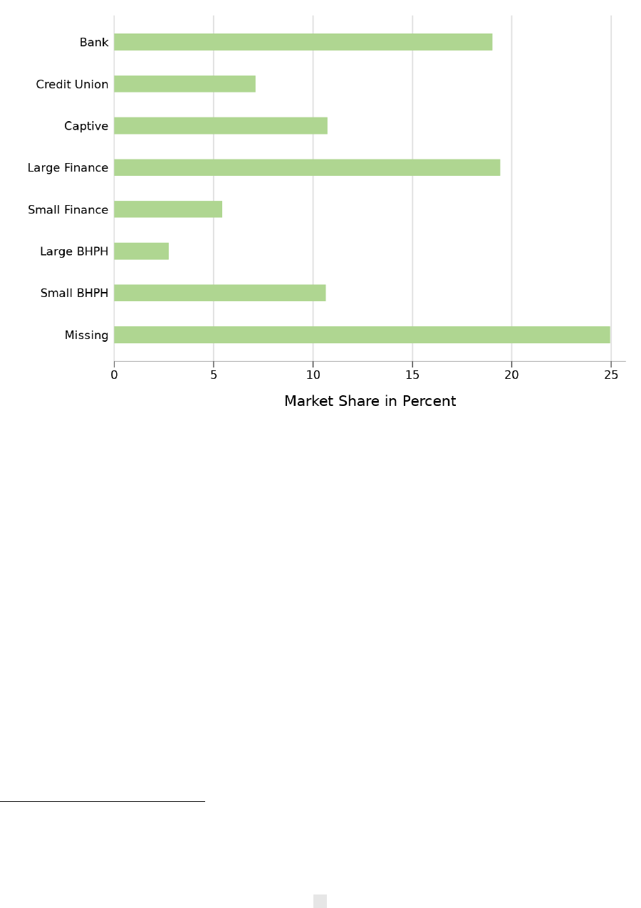
FIGURE 1: SUBPRIME MARKET SHARE BY LENDER TYPE
Next, we study, to the extent possible, how borrowers, loans, and vehicles differ across lender
types in the AutoCount® data. Recall that the AutoCount® data are not at the individual-loan
level, but instead are aggregated to the dealer-lender-month-(new or used vehicle)-(credit score
bin) level. Out of necessity, for every variable we treat every observation in a bin as having the
observed mean of that variable in that bin. For example, one bin with ten loans may have five
loans securing a vehicle worth $7,500 and five loans securing a vehicle worth $12,500. We only
observe that the average vehicle value in that bin is $10,000, and so the analysis below will treat
the data as if every vehicle in that bin is worth $10,000.
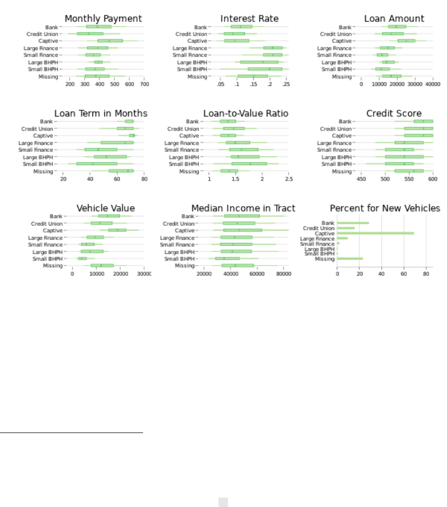
We begin with AutoCount® data that are available for all observations whether information on
the loans is furnished or not: bin-level observations of credit score, vehicle value, and the
percent of loans for new vehicles, as well as the median household income in the dealer’s (not
borrower’s) census tract.
23
For most variables, Figure 2 shows the 25
th
to 75
th
percentiles (thick
23
AutoCount® has data on the dealer’s zip code, which is matched to data on income by census tract from
the American Community Survey. Our AutoCount® data do not have information on borrowers’ income
or locations.
14

boxes) as well as the 10
th
and 90
th
percentiles (thin boxes)and the median (dark green line).
24
The figure also shows the percent of loans that are for new vehicles at each type of lender.
FIGURE 2: SUBPRIME LOAN OBSERVABLES BY LENDER TYPE
Figure 2 shows that there are substantial differences in borrowers and vehicles across lender
type. Vehicles securing subprime loans from Captives are notably different from other vehicles:
they are typically more valuable and are much more likely to be new. Bank and Credit Union
borrowers typically have higher credit scores than Finance and BHPH borrowers, and their
loans are for more valuable vehicles. Small Finance and Small BHPH borrowers have even lower
credit scores and buy less valuable cars than Large Finance and Large BHPH borrowers. Data on
income in dealers’ census tracts are a noisy measure of borrowers’ creditworthiness, but they
also indicate that Small Finance and Small BHPH borrowers are in general less creditworthy
than other borrowers.
24
Recall that credit scores are in bins of 20: 600-619, 580-559, etc. The figure shows the lower bound for
a bin, and consumers with credit scores above 619 are not considered subprime and so are not included in
the figure. Therefore 600 is the highest value in the data for subprime consumers. This is why it is the
highest value shown in Figure 2 as well as why so many Bank, Credit Union, and Captive borrowers have
that value in the data.
15

However, there is also some overlap in the distributions. For example, the 90
th
percentile of
Small Finance and Small BHPH borrowers have significantly higher credit scoresthan the 10
th
percentile of Bank and Credit Union borrowers. This may indicate that some Finance and BHPH
borrowers could have obtained loans instead from a Bank or a Credit Union. It may also indicate
that some Finance and BHPH borrowers are genuinely comparable to some Bank and Credit
Union borrowers, which is important for interpreting results presented later.
4.2. Comparing furnished and non-furnished loans
As already discussed, the AutoCount® data have several other informative variables, but these
are only available for furnished loans. The CCP, used later, also only has data for furnished
loans. Therefore, we now turn towards understanding, to the extent possible, how furnished
loans differ from loans that are not furnished, and how this varies across lender types.
In the AutoCount® data we observe the number of auto loans in each bin as well as the number
of auto loans successfully matched to an auto loan on a credit record. The ratio of the latter to
the former should be a good proxy for the fraction of auto loans that were furnished.
25
Figure 3
below shows the percent of subprime loans “furnished” by lender type, where “furnished” is
defined using the proxy.
25
A match could be unsuccessful, even if the data are furnished, if the data are not furnished by the time
the match is attempted or if the data are not furnished correctly (e.g. the loan is reported as an installment
loan and not an auto loan). Appendix A examines furnishing delays and how they may affect successful
match rates.
16

FIGURE 3: PERCENT OF SUBPRIME LOANS “FURNISHED” BY LENDER TYPE
Consistent with conventional wisdom, Banks, Credit Unions, and Captives all furnish data at
very high rates. As discussed in Appendix A, for these lender types furnishing delays appear able
to explain nearly all of the failed matches in our proxy, meaning that for these lender types
furnishing rates are nearly 100 percent. However, again consistent with conventional wisdom,
Small Finance and Small BHPH lenders furnish at far lower rates.
The very low furnishing rates of Small Finance and Small BHPH lenders means that loans
furnished by those lender types may differ in important ways from all loans originated by those
lender types. To understand how furnished loans differ from all loans for Small Finance and
Small BHPH borrowers, Figure 4 shows the 25
th
to 75
th
percentiles (thick boxes) as well as the
10
th
and 90
th
percentiles(thin boxes)and the median (dark green line) of the same variables as
in Figure 2.
26
Because Figure 3 showed that loans from Large Finance (BHPH) lenders are far
more likely to be furnished than loans from Small Finance (BHPH), Figure 4 also shows this
26
Figure 4 does not show the percent of loans for new vehicles because very few loans from Small Finance
and Small BHPH lenders are for new vehicles, whether they are furnished or not. Only roughly 2 percent
and .6 percent of furnished loans for Small Finance and Small BHPH lenders, respectively, are for new
cars. For all loans from Small Finance and Small BHPH lenders, the numbers are .7 percent and .1
percent, respectively.
17

information for lender size in annual loan volume. Again, recall that the AutoCount® data are
not at the individual loan level, but instead are aggregated to the dealer-lender-month-(new or
used vehicle)-(credit score bin) level. This means that Figure 4 examines differences in
observable characteristics across bins, but not within them.
FIGURE 4: SUBPRIME LOAN OBSERVABLES BY FURNISHED STATUS
Figure 4 shows that furnished loans tend to be for higher credit score consumers and for more
valuable cars. Therefore, in the analysis that follows using furnished loans, our sample of Small
Finance and Small BHPH borrowers is likely to be more creditworthy than Small Finance and
Small BHPH borrowers overall. Perhaps surprisingly, while as shown in Figure 3 loans from
Large Finance (BHPH) lenders are far more likely to be furnished than loans from Small
Finance (BHPH) lenders, within Small Finance and Small BHPH loans it does not appear to be
the case that furnished loans are from larger lenders than non-furnished loans.
18
4.3. Studying furnished loans in AutoCount®
Next, we study how all variables available in the AutoCount® data vary by lender type,
weighting bins by the number of furnished loans they contain. For most variables, Figure 5
shows the 25
th
to 75
th
percentiles (thick boxes) as well as the 10
th
and 90
th
percentiles (thin
boxes) and the median (dark green line).
27
The figure also shows the percent of loans that are for
new vehicles at each type of lender.
FIGURE 5: SUBPRIME LOAN OBSERVABLES FOR FURNISHED LOANS BY LENDER TYPE
Figure 5 shows that, even focusing on borrowers with loans that are furnished, Bank and Credit
Union borrowers in general appear more creditworthy than Finance and BHPH borrowers. For
example, they have higher credit scores and lower LTVs. However, there is also overlap in the
distributions. For example, the 90
th
percentile of Small Finance and Small BHPH borrowers
have credit scores about 60 points higher than the 10
th
percentile of Bank borrowers. There are
27
Recall that credit scores are in bins of 20: 600-620, 580-600, etc. The figure shows the lower bound for
a bin, and consumers with credit scores above 620 are not considered subprime and so are not included in
the figure. Therefore 600 is the highest value in the data for subprime consumers.
19

also substantial differences in interest rates across lender types. Later we will explore the extent
to which these differences in interest rates can be explained by differences in default risk.
4.4. Studying furnished loans in the CCP
Finally, we examine how observables differ across lender types in the CCP. Recall that the CCP is
constructed from information furnished by lenders and so includes only furnished loans.
28
Unlike AutoCount®, data in the CCP are available at the individual-loan level. Figure 6 shows
the 25
th
to 75
th
percentiles (thick boxes) as well as the 10
th
and 90
th
percentiles (thin boxes) and
the median (dark green line) of selected variables. The figure also shows the percent of
borrowers at each type of lender that have mortgages, as well as the percent of borrowers with a
co-borrower or co-signer.
28
The CCP does not separately identify captives from other finance companies. Captives are notable for
being large and for offering a large number of loans at very low interest rates. Therefore, we define
captives in the CCP as finance companies that are in the top 100 by market share and with at least 5
percent of loans with an interest rate of less than 1 percent.
20

FIGURE 6: SUBPRIME LOAN OBSERVABLES BY LENDER TYPE IN THE CCP
Figure 6 shows again that Bank and Credit Union subprime borrowers are generally more
creditworthy than Small Finance and Small BHPH subprime borrowers. However, again there is
overlap in the distributions. A large number of Small BHPH borrowers are measured to have
very low interest rates, which may be a data or credit reporting issue.
29
However, it may also in
part reflect that BHPH dealerships, unlike other lender types, control the price of the vehicle as
well as the interest rate on their loan. In many cases BHPH dealerships may be indifferent
between charging consumers for the car or the loan and so may charge a below-market interest
rate in exchange for an above-market vehicle price.
30
29
The interest rate issue appears to exist in the AutoCount® data too. In that data, the 5
th
percentile of
interest rates for Banks, Small Finance, and Small BHPH loans is .05, .04, and .01, respectively. However,
the AutoCount data are aggregated into bins while the CCP data are not, which may explain why the CCP
data include more surprisingly low interest rates.
30
For evidence that BHPH dealerships do sometimes charge a comparatively low interest rate in exchange
for a high vehicle price, see Brian Melzer and Aaron Schroeder, 2017, “Loan Contracting in the Presence of
Usury Limits: Evidence from Automobile Lending”, available at
https://papers.ssrn.com/sol3/papers.cfm?abstract_id=2919070.
21

5. Are interest rates explained
by default risk?
Section 4 showed that there are large differences in the interest rates charged by different types
of auto lenders. Since interest payments might compensate lenders for default risk, one
hypothesis is that these differences can be entirely explained by differences in the default risk of
loans across lender types. This section examines this hypothesis. Other possibilities, such as
that different lender types evaluate risk in different ways or that different lender types suffer
different losses from default, are discussed in Section 6. Since borrowers’ ex-ante default risk is
unobservable, we use borrowers’ ex-post default outcomes to proxy for it.
31
As described in
Section 3, delinquency is measured roughly 38 months after origination.
5.1. Defining “default risk” in our data
In the CCP an auto loan may be delinquent in many ways, ranging from 30-day delinquency to
terminated with a repossession. Borrowers who become 30-days delinquent typically make up
their delinquent payment and get current again with almost no loss to the lender, and so 30-day
delinquency may not be useful for studying the effects of default risk on interest rates. More
serious measures of delinquency could imply greater expected losses for the lender and so likely
have a greater impact on interest rates, but they have the disadvantage that they reflect not only
the probability that a borrower becomes delinquent but also the lender’s behavior in response to
that delinquency. For example, one lender may prefer to cooperate with delinquent borrowers to
maximize the chance they become current on their own. Another lender may prefer to repossess
vehicles quickly. Even if these two lenders have borrowers that are otherwise identical, loans
from the latter lender are likely to ultimately end in repossessions at a higher rate if
repossessions have a causal negative effect on the probability a delinquent borrower becomes
31
For a discussion of how one large subprime auto lender uses default outcomes to predict default risk,
see Mark Jansen, Hieu Nguyen, and Amin Shams, 2021, “Rise of the Machines: The Impact of Automated
Underwriting”, available at https://papers.ssrn.com/sol3/papers.cfm?abstract_id=3664708. For a recent
discussion of how economists use default outcomes to proxy for default risk when studying discrimination
in lending markets, see Alexander W. Butler, Erik J. Mayer, and James Weston, 2021, “Racial
Discrimination in the Auto Loan Market”, available at
https://papers.ssrn.com/sol3/papers.cfm?abstract_id=3301009.
22

and stays current.
32
In Section 6, we present suggestive evidence that different lender types
respond to borrower default in different ways, and so this is an important issue.
To balance these concerns, we investigate two specific definitions of default. We define “60-day+
delinquency” as a borrower everexperiencing 60-day delinquency or anything worse, i.e.
including voluntary and involuntary vehicle repossessions, chargeoffs, collections, and
bankruptcies.
33
This definition of default is useful because lenders rarely initiate vehicle
repossessions before a borrower becomes at least 60 days delinquent. Therefore, 60+ day
delinquency is a useful outcome measure that is determined mostly by borrower behavior. The
other definition of default we consider is 90-day+ delinquency, which we define as a borrower
everexperiencing 90-day delinquency or anything worse. This definition is useful because most
lenders will consider a loan that is 90 days delinquent to be in serious trouble and likely not to
be paid in full. The choice whether to work with the borrower and hope they can become current
on the loan, to repossess the vehicle, to initiate collections, etc. will vary from lender to lender as
well as from borrower to borrower. Therefore, the disadvantage of 90-day+ delinquency is that
it is in part a measure of lender behavior as well as borrower’s creditworthiness.
34
However, the
advantage of 90-day+ delinquency is that it is likely more useful from the lender’s underwriting
perspective. Many loans that become 60 days delinquent are ultimately paid in full.
In this section we study auto loan default rates (an ex-post measure of loan performance that we
observe) to learn about auto loan default risk (an ex-ante measure of expected loan performance
that we do not observe). However, if the macroeconomic environment deteriorates rapidly and
unexpectedly (as it did at the beginning of the COVID-19 crisis), then borrowers will likely
default at higher rates than their default risk, evaluated ex-ante, would indicate. This is the
main reason that in this report we only study auto loans originated between 2014 and 2016; this
restriction ensures we study auto loan performance between 2014 and 2019, a generally stable
macroeconomic period in which actual macroeconomic performance did not deviate
substantially from expectations. During this period auto loan default rates are likely a very good
proxy for auto loan default risk, but this caveat should be kept in mind.
32
For evidence that repossessions after delinquency have a negative causal effect on borrowers’ future
credit outcomes, see Elizabeth Berger, Alexander W. Butler, andE rik J. Mayer, “Credit Where Credit Is
Due: Drivers of Subprime Credit”, 2018, available at http://dx.doi.org/10.2139/ssrn.2989380.
33
A “voluntary repossession” occurs when the borrower returns the vehicle to the lender, perhaps in
response to communications from the lender. An “involuntary repossession” occurs when the lender,
possibly through a third party, repossesses the vehicle without the permission of the borrower.
34
This is also why we include e.g. a borrower who becomes 60-days delinquent and becomes current in
our measure of 60-day+ delinquency. For example, if borrowers A and B in that group have identical
probabilities of becoming current on their own, but borrower A’s vehicle is repossessed quickly by the
lender and B’s is not, it would otherwise appear that borrower A was riskier.
23

5.2. How does default risk vary across lender types?
Subprime auto loans carry substantial default risk; roughly 27 percent of our subprime CCP
sample is 60-day+ delinquent. Different lender types specialize in different amounts of default
risk. Finance companies and BHPH dealerships typically specialize in the riskiest loans, while
Banks and Credit Unions generally specialize in the least risky loans. Therefore, we would expect
delinquency rates to vary across lender type.
First, we examine how 60-day+ delinquency risk varies across lender type. We are interested in
understanding whether delinquency risk varies across characteristics we can observe in the CCP
(such as credit score), as well as across characteristics we cannot observe (such as income).
Therefore, Figure 7 plots 60-day+ delinquency risk by lender type, in three ways.
The green dots plot unconditional default rates by lender type. The figure shows that there is
considerable variation in default rates across lender types, and that this variation is mostly as
expected. For example, the figure shows that the 60-day+ delinquency rate for Small Finance
borrowers in the sample is very high, nearly 40 percent. For bank borrowers, it is only slightly
more than 15 percent. Large BHPH borrowers and Small Finance borrowers are comparable in
default risk to each other and are substantially riskier than Small BHPH borrowers and Large
Finance borrowers, who are comparable in risk to each other and to Captive borrowers. It is
likely that the comparatively low default rate of Small BHPH borrowers is at least partly due to
the fact that Small BHPH borrowers whose loans are furnished are less risky than Small BHPH
borrowers overall (see Figure 4). However, Small Finance borrowers whose loans are furnished
are also less risky than Small Finance borrowers overall (again, see Figure 4), making their
comparatively high default rate more of a puzzle. Bank and Credit Union borrowers have the
lowest default rates.
The orange dots plot our average predicted 60-day+ delinquency rates after accounting for
differences in control variables by lender type.
35
For example, the decline in 60+ day
delinquency rates for Small Finance borrowers from roughly 40 percent without controls to
roughly 30 percent with controls means that the regression predicts that the default rates for
Small Finance borrowers would fall by roughly 10 percentage points, if instead of having the
observables that Small Finance borrowers have in the data (such as credit score), Small Finance
35
We used a logit regression to predict delinquency rates. The logit model is described in Appendix B. The
controls in the regression include credit score, age, whether the borrower has a mortgage on their credit
report, whether there is a co-borrower or co-signer on the loan, and lender type fixed effects. We also
considered including credit scores from previous years, the logarithm of median household income in the
borrower’s census tract, the percent of people in the borrower’s census tract with high school and college
degrees, and local market shares of the various lender types in the regressions, but these controls are not
available for all observations so we do not include them.
24

borrowers had the observables that all borrowers have in the data. Our controls explain some
but not most of the variation in default risk across lender types in the data. Potential
explanations for the remaining variation in default risk across lender types include (but are not
limited to) differences in income levels, income variation, down payments, access to liquid
assets, access to other forms of credit, financial sophistication and defaults costs across
borrowers, differences in business practices when originating and servicing loans across lenders,
and differences in quality and depreciation rates across financed vehicles.
The blue dots are the same as the orange dots, except restricting both the regression and the
sample to consumers with credit scores of at least 560 (“shallow subprime”). For example, the
regression predicts that the 60-day+ delinquency rate for the Small Finance borrowers in our
shallow subprime sample would be around 28 percent if they had the observables of all shallow
subprime borrowers in the data and not of shallow subprime Small Finance borrowers.
Restricting the sample to shallow subprime borrowers, and including control variables, explains
enough of the variation for comparisons across lender types to be meaningful. With controls,
shallow subprime Small BHPH borrowers appear comparable in default risk to shallow
subprime Bank and Credit Union borrowers, while shallow subprime Small Finance and Large
BHPH borrowers appear comparable in default risk to shallow subprime Large Finance
borrowers. However, even in the shallow subprime market, borrowers from Captives, Large
Finance, Small Finance, and Large BHPH lenders appear to be significantly riskier than Bank
and Credit Union borrowers for reasons we cannot observe in the CCP.
Our regressions account for uncertainty in our findings. In the figures, the bands around the
dots indicate 95 percent confidence intervals. For example, roughly speaking, our regression is
95 percent confident that the 60-day+ delinquency rate for the Small Finance borrowers in our
shallow subprime sample would be between about 25-31 percent if they had the observables of
all shallow subprime borrowers in the data and not of shallow subprime Small Finance
borrowers.
36
36
A more formal definition of these confidence intervals is as follows. Suppose we were to repeat the
procedure in Figure 7 N times, where N is a natural number, each time usinga different dataset that is
equivalent in size and quality to the one we use. For each estimate shown (e.g. the 60-day+ delinquency
rate for shallow subprime Small Finance borrowers if they had the observables of all shallow subprime
borrowers in our data), each repetition of the procedure would yield a different confidence interval,
because of the different data used. Then, under the assumptions used in the logit model (described in
Appendix B), asN grew larger and larger the percent of confidence intervals calculated in this way that
included the true, unknown value being estimated would approach 95 percent.
25

FIGURE 7: 60-DAY+ DELINQUENCY RISK BY LENDER TYPE
Figure 7 suggests that, when compared to the raw data, default risk does not vary as much
across lender types when we condition on the variables we can observe. However, they do not
show whether observationally similar borrowers do indeed obtain loans from different lender
types. For example, it could be the case that all Small BHPH borrowers are observably riskier
than all Bank borrowers. Next, we investigate whether this is true.
Figure 8 plots the cumulative density functions of estimated 60-day+ delinquency risk by lender
type.
37
For a given level of default risk (on the x-axis), the cumulative density (on the y-axis)
shows the estimated fraction of borrowers at that lender type with lower default risk. For
example, the figure shows that over 90 percent of Credit Union borrowers are estimated to have
less than a 20 percent chance of 60+ day delinquency, while fewer than 5 percent of Small
Finance borrowers do.
37
We use a logit regression with the same controls as before to predict 60+ day delinquency. The logit
model is described in Appendix B. Note that these controls include lender fixed effects, which should
effectively control for delinquency risk that varies across lender types for reasons we do not observe.
26

FIGURE 8: DISTRIBUTION OF PREDICTED DEFAULT RISK, BY LENDER TYPE
There are large and predictable differences in the distributions. Bank and Credit Union
customers on average have the lowest default risk. All of the other lender types appear to
provide loans to many consumers with a default risk greater than 20%, who would likely have
difficulty obtaining a loan from a Bank or Credit Union. Small Finance and Large BHPH
customers are the highest risk. Large Finance companies appear to have large numbers of
customers with both fairly low and fairly high risk. However, there is also substantial overlap in
the distributions. For example, roughly 30 percent of Small BHPH borrowers have estimated
default risk less than 20 percent; roughly 20 percent of Bank borrowers have estimated default
risk above this number. This may indicate that many of these less risky Small BHPH borrowers
could have obtained a loan from a Bank. Similarly, many Large BHPH and Small Finance
borrowers appear less risky than many Large Finance borrowers.
5.3. How do interest rates vary across lender types?
As shown in Figures 5 and 6, subprime auto loans vary substantially in their interest rates. High
interest rates may compensate lenders for bearing risk, and so higher-risk consumers should be
27

expected to pay higher interest rates. Figures 7 and 8 show that there are large differences in
consumers’ default risk across lender type. Lenders with higher-risk borrowers should be
expected to charge those borrowers higher interest rates, and so interest rates should vary with
default risk across lender types. However, interest rates may also vary across lender type for
reasons besides default risk. Potential reasons for this variation include (but are not limited to)
other prices relevant to borrowers (such as the price of the vehicle), borrowers’ bargaining
power and financial sophistication, lenders’ losses from delinquency, underwriting ability, and
willingness and ability to extract revenue from borrowers, and (for indirect loans) dealers’
willingness and ability to mark up loan interest rates over and above what the lender is willing to
offer.
Next, we investigate how interest rates vary across lender types. Figure 9 performs the same
analysis as Figure 7, but with interest rates as the outcome of interest rather than default rates.
38
Because default is not the outcome variable, we can now also include actual default outcomes in
the regression. Here we are most interested in the default risk that lenders use for underwriting,
so we use 90-day+ delinquency risk rather than 60-day+ delinquency risk. Controlling for actual
default outcomes provides evidence on whether variation in 90-day+ delinquency risk that
cannot be explained by the default regression, which could for example arise from unobserved
differences in borrower incomes or vehicle values, can explain variation in interest rates. The
fourth set of points, colored brown, does this for the shallow subprime sample.
38
Since interest rates (a continuous variable) are the outcome of interest, rather than delinquency (a
binary variable), we run an Ordinary Least Squares (OLS) regression rather than a logit regression to
predict interest rates. The OLS model is described in Appendix C.
28

FIGURE 9: INTEREST RATES BY LENDER TYPE
Interest rates vary with default risk across lender types in some ways that are intuitive. Bank
and Credit Union borrowers, who are the least risky, pay the lowest interest rates. However,
some differences in interest rates across lender types do not seem to be fully explained by
default risk. Captive borrowers pay interest rates comparable to those of Bank and Credit Union
borrowers, despite having default risk comparable to those of Large and Small Finance
borrowers. This may be because their loans are often secured by newer and more valuable
vehicles, or because the business model of captives is, in part, to subsidize loans in order to
increase vehicle demand.
39
Even though shallow subprime Small BHPH borrowers have similar
risk to observationally comparable Bank and Credit Union borrowers, they pay notably higher
interest rates. Similarly, shallow subprime Small Finance and Large BHPH borrowers pay
substantially higher interest rates than observationally similar Large Finance borrowers, even
though their default risk is comparable. These statements are true even after controlling for
actual default outcomes, as the brown points do. In general, variables we can observe in the data
39
We showed in Section 4 that vehicles securing loans from captives are in general more valuable than
vehicles securing loans from other lender types at the time the vehicle is purchased. What matters for the
pricing of delinquency risk is vehicle value at the time of default, not at the time of purchase, because this
is what affects the lenders’ losses from delinquency. It seems likely that vehicles securing loans from
Captives are also more valuable than other vehicles at the time of default, though we cannot test this.
29

explain less of the variation in interest rates than the variation they explain in default rates. This
suggests that interest rates may vary across lender types for reasons beyond default risk.
The differences in interest rates shown in Figure 9 are quantitatively large. A borrower with the
median loan term and loan amount for Small BHPH borrowers in AutoCount® would save
roughly $894 over the life of a loan if she could reduce her interest rate from 13 percent (roughly
the brown point for Small BHPH borrowers) to nine percent (roughly the brown point for Bank
borrowers). A borrower with the median loan term and loan amount for Small Finance
borrowers in AutoCount® would save roughly $1,348 over the life of a loan if she could reduce
her interest rate from 18 percent (roughly the brown point for Small Finance borrowers) to 13
percent(roughly the brownpoint for Large Finance borrowers.)
40
40
As noted in the introduction, this estimate does not necessarily imply that a specific borrower could
save $1,348 by switching lender types because these estimates are not causal and there are variables we do
not observe and so cannot control for (such as financing fees).
30

6. Discussion and suggestions
for future research
The previous section provided evidence that there is variation in interest rates across lender
types that cannot be explained by default risk. This raises a critical question: why else do
interest rates vary across lender types? The limitations of our data mean we must leave a
definitive answer to this question to future research. But this section discusses potential
explanations for our results and provides some useful clues to distinguish between them.
6.1. Some potential explanations for variation in
interest rates
An important possibility for why interest rates vary across lender types is that a given level of
default risk poses a greater risk to, for example, the profits of Small BHPH lenders than it does
for Banks. For example, more Bank borrowers that are 90+ days delinquent could still become
current than otherwise comparable 90+ day delinquent Small Other borrowers. Moreover, in
Section 4 we showed in the AutoCount® data that the vehicles securing Small BHPH loans are
in general less valuable at loan origination than the vehicles securing Bank loans. This may
mean that vehicle repossessions may recover less of the loan amount for Small BHPH lenders
than for Banks.
41
Small BHPH lenders may also recover less from consumers in collections than
Banks do. Repossessions or collections could be more expensive for Small BHPH lenders to
initiate than Banks, perhaps because their borrowers are more difficult to find after default or
because of local regulations. If any of the above are true, the loss given default for Small BHPH
lenders could be higher than it is for Banks. Therefore, a given level of delinquency would pose
more of a risk to Small BHPH lenders than to Banks, which in turn could explain why Small
BHPH borrowers pay higher interest rates than Bank borrowers with similar default risk. If this
kind of explanation is true, then it would have an empirical implication we can test in our data:
the difference between the interest rates paid by risky and less risky borrowers should be greater
for Small BHPH lenders than it is for Bank lenders.
A different set of explanations come from underwriting practices and funding structure. As
shown in Section 4, Banks and Credit Unions typically focus on the higher end of the subprime
41
Note in the previous section we could not control for vehicle value because it is not in the CCP data.
31

credit spectrum, which could mean they have the underwriting ability to separate risky
borrowers from less risky borrowers. Moreover, they typically hold the loans they originate, and
so may place greater value on low-risk loans. Conversely, as noted above, many Finance and
BHPH lenders explicitly advertise their willingness to lend to borrowers who appear quite risky.
This could give them less incentive to invest in underwriting to separate risky borrowers from
less risky borrowers, since they will lend to risky borrowers anyway, and so they may not be able
to offer lower interest rates to less risky consumers because they cannot identify them. BHPH
lenders profit from selling vehicles as well as financing them, so if a delinquency results in a
repossession, this gives them another chance to sell the vehicle which in turn may lower the loss
given default. Moreover, Finance and BHPH lenders often adopt technologies such as GPS
tracking devices and starter-interrupt devices that lower their costs when consumers default,
42
and these lenders may optimize their funding structure for the deep subprime market they
specialize in. These factors could raise the cost of issuing and servicing loans for consumers that
are not particularly risky but reduce the cost of issuing and servicing loans for especially risky
consumers. Finance and BHPH lenders may also have little incentive to offer their less risky
customers lower interest rates, since they may assume that if the consumer has approached
them that means they will be willing to pay the interest rates associated with riskier borrowers.
If this kind of explanation is true, then for example the difference between the interest rates paid
by risky and less risky borrowers should be smaller for Small BHPH lenders than it is for Banks.
Finally, interest rates may vary across lender types for reasons that have nothing to do with
delinquency risk. As depository institutions, Banks and Credit Unions have may have access to
cheaper funding than Finance or BHPH lenders, and so may be able to provide all customers
lower interest rates. If there are returns to scale in auto lending, then larger institutions may be
able to provide loans more efficiently and thus at lower interest rates than smaller institutions.
43
Captives and BHPH dealerships have financial incentives to originate loans beyond the interest
payments they generate, so they may simply offer more competitive interest rates for all
consumers in order to sell more vehicles. If this kind of explanation is true, then for example the
difference between the interest rates paid by risky and less risky borrowers should be roughly
the same for Small BHPH lenders as it is for Banks.
42
For example, see https://www.forbes.com/sites/kashmirhill/2014/09/25/starter-interrupt-
devices/#5466b0b07733.
43
For some evidence that this may be the case, see Constantine Yannelis and Anthony Lee Zhang, 2021,
“Competition and Selection in Credit Markets”, available at
https://anthonyleezhang.github.io/pdfs/competitionselection.pdf.
32

6.2. Delinquency risk premia by lender type
Section 6.1 provided a long, but not exhaustive, list of potential explanations for differences in
interest rates across lender types. Definitively distinguishing between these explanations is well
beyond what is possible in our data. However, as discussed in Section 6.1, these various
explanations can be placed into categories based on whether they predict that the difference in
interest rates paid by risky borrowers and less risky borrowers should be larger, smaller, or the
same across lender types. This is something we can investigate in our data.
To investigate which kind of explanation more closely fits the data, Figure 10 plots average
predicted interest rates, assuming borrowers have the lender type and ultimate delinquency
status shown, but the other observable characteristics of borrowers in the shallow subprime
sample.
44
For example, the figure shows that the average predicted interest rate for shallow
subprime Bank borrowers, if they had the observable characteristics of borrowers in the shallow
subprime sample and would not ultimately become delinquent, is roughly nine percent. The
figure also shows that the average predicted interest rate for shallow subprime Bank borrowers,
if they had the observable characteristics of borrowers in the shallow subprime sample and
would ultimately become delinquent, is roughly 11 percent. This is an indication that Banks
charge borrowers higher interest rates if they are riskier for reasons that are not observable in
our data. Captives and Large Finance companies also appear to charge borrowers higher interest
rates if they are riskier for reasons that are not observable in our data. By contrast, the interest
rate premium paid by borrowers at Credit Unions, Small Finance companies and BHPH lenders
(especially Small BHPH lenders) who ultimately become delinquent, relative to those who do
not ultimately become delinquent, is smaller. However, because Small BHPH lenders furnish at
very low rates as shown in Figure 3, the sample of Small BHPH loans in the data is not large and
so there is some uncertainty around this result for Small BHPH borrowers.
44
The OLS regressionis exactly the same as that used for the brown dots in Figure 8, except it does not
have separate fixed effects for lender type and delinquency status, but instead has fixed effects for lender
type interacted with delinquency status. The OLS model is described in Appendix C.
33

FIGURE 10: INTEREST RATES BY LENDER TYPE AND DEL
Figure 10 shows that the interest rate premium paid by borrowers who became delinquent,
relative to borrowers who did not become delinquent, is smaller (or at least not larger) at Small
Finance, Large BHPH, and Small BHPH lenders than at other lenders. This is suggestive
evidence in favor of the second and third category of explanations discussed in Section 6.1 for
the interest rates charged by these lender types, and against the first category of explanations
which predict that default is particularly costly for these kinds of lenders.
6.3. Servicing after delinquency by lender type
Next, we investigate how different lender types service delinquent loans. This may provide
another useful, if imperfect, method for distinguishing between the categories of explanations
discussed in Section 6.1. For example, if repossessions are more (less) difficult or expensive for
some lender types, then those lender types may be slower (faster) to repossess a vehicle after a
borrower becomes delinquent.
34

For this purpose, we restrict our attention to borrowers who ever become at least 30-days
delinquent on a loan, and we focus on the first time they do so. The goal is to examine whether,
two months after this delinquency, different lender types have either repossessed the vehicle or
started collections at different rates. We drop borrowers who are less than 90-days delinquent
two months after becoming 30-days delinquent, and place the remaining loans into one of four
categories: (1) still delinquent, (2) terminated by the borrower (through bankruptcy or a
voluntary repossession), (3) terminated by the lender through chargeoff or collections, and (4)
terminated by the lender through involuntary repossession of the vehicle.
45
Figure 11 shows the
percent of loans in each category by lender type.
FIGURE 11: LOAN STATUS TWO MONTHS AFTER FIRST DELINQUENCY
Figure 11 shows that Captives, Small Finance and Small BHPH lenders appear to terminate
delinquent loans more quickly than Banks or Credit Unions. For example, of loans that were at
least 90-days delinquent two months after becoming 30-days delinquent, nearly 30 percent of
45
Accounts can transition from bankruptcy or repossession to chargeoff or collections, if the lender
recovers less than the total loan amount outstanding. However, few accounts transition from 30-days
delinquent to bankruptcy or repossession, which means that this kind of transition rarely affects account
status two months after an account first becomes 30-days delinquent.
35

Small BHPH loans were terminated through an involuntary repossession while less than 20
percent of Bank loans were. Broadly, Figure 11 supports the same conclusion as Figure 10: loans
terminating in default do not appear to be more costly for lender types that charge higher
interest rates. Clearly, however, much more research on this topic is necessary.
36

7. Conclusion
This report shows that there are large differences in the auto loan borrowers served by different
lender types. For example, Banks and Credit Union customers are on average notably more
creditworthy, and pay lower interest rates, than Small Finance and Small BHPH borrowers.
However, there is also overlap in the distribution of observables across lender types. There are
Small Finance borrowers and Small BHPH borrowers that appear comparable to many Bank
and Credit Union borrowers.
We investigated the extent to which differences in borrower creditworthiness across lender
types could explain the differences in borrowers’ interest rates across lender types. After
controlling for the borrower characteristics that we observe, we found that Small BHPH
borrowers appeared comparable in default rates to Bank and Credit Union borrowers, while
Small Finance and Large BHPH borrowers appeared comparable in default rates to Large
Finance borrowers. However, Small BHPH borrowers still paid substantially higher interest
rates than observationally similar Bank and Credit Union borrowers. Small Finance and Large
BHPH borrowers paid substantially higher interest rates than observationally similar Large
Finance borrowers.
There are many potential explanations for these findings. While we cannot definitively
distinguish between them with our data, we described three classes of explanations for our
findings. First, a given amount of default risk could be more costly for one kind of lender than
another. Second, some lender types may differentiate between comparatively low-risk and high-
risk borrowers more than other lender types. Third, some lender types may be able to provide
better interest rates for their borrowers, regardless of default risk, than other lender types. We
present some suggestive evidence that provides more support for the latter two classes of
explanations.
This report sheds valuable light on an important market, but it has several limitations.
Addressing these could be a valuable path for future research. One limitation is that the results
we find are descriptive and do not establish a causal relationship. For example, we found that
Small BHPH borrowers pay higher interest rates than observationally similar Bank borrowers.
This could mean that these Small BHPH borrowers would have paid lower interest rates had
they obtained their loans from Banks. However, this relationship might also arise if, for
example, Small BHPH lenders attract borrowers who are not focused primarily on interest rates
and that Banks would also charge these borrowers relatively high rates.
Another important limitation is that, while we do observe interest rates and delinquency
outcomes, we do not observe many other factors that may be relevant for auto loan borrowers.
37

For example, borrowers often must pay substantial fees to obtain auto loans, and we cannot
study how fees vary across lender types. There are many other loan characteristics we cannot
study. For example, it is also possible that borrowers seek to avoid the negative consequences
associated with a denial of credit and so may be willing to pay an interest rate premium in order
to minimize the chances of being denied.
Together, these results and their limitations call for more research on auto loan borrowers’
objectives, how they shop for auto loans, and how their objectives and shopping behavior
influence borrower and loan outcomes.
38

APPENDIX A:
Furnishing delays by lender
type and credit score:
Lenders sometimes take weeks or months after a loan is originated to begin furnishing
information on that loan to the NCRAs. Both the AutoCount® and CCP data studied in this
report are created from furnished information and so may be affected by these furnishing
delays.
To investigate how these delays may affect our results, we study the CCP data used in the main
body of this report. Recall that, as described in Section 3, these data include only subprime auto
loans. Thus, the analysis in this appendix covers only subprime auto loans.
For every quarter in our data except the first (i.e. excluding 2014Q1), we examine the percent of
loans in the data that are also in data from the previous quarter, conditional on whether they
were originated in the first or second month of that quarter. For example, we study the percent
of loans in the 2014Q2 data that are also in the 2014Q1 data, conditional on whether they were
originated in January 2014 or February 2014. Loans will appear in the 2014Q1 data if they were
furnished by the time the data was constructed, roughly in March 2014. If lenders begin
furnishing loan information by around eight weeks after loan origination, then loans originated
in January 2014 will appear in the 2014Q1 data. However, loans originated in February 2014
will only appear in the 2014Q1 data if lenders begin furnishing loan information by around four
weeks after loan origination. To the extent that nearly all loans that will ever be furnished are
furnished within 16 weeks of origination, then the 2014Q2 data should include nearly all loans
originated in January or February 2014 that will ever be furnished. Thus, restricting attention to
loans originated in January (February) 2014, the fraction of loans in the 2014Q2 data that are
also in the 2014Q1 data provides a rough proxy for the fraction of loans that will eventually be
furnished that are actually furnished within eight (four) weeks of loan origination. Finally,
restricting attention to loans originated in either January or February, the fraction of loans in
the 2014Q2 data that are also in the 2014Q1 data provides a rough proxy for the fraction of loans
39

that will eventually be furnished that are actually furnished within four to eight weeks of loan
origination.
Figure A1 shows the results from this exercise, by lender type and credit score bin. The orange
dots show our estimate of the percent of loans that will eventually be furnished within roughly
sixteen weeks of origination that are actually furnished within roughly four weeks. The blue dots
show our estimate of the percent of loans that will eventually be furnished within roughly
sixteen weeks of origination that are actually furnished within roughly eight weeks. The green
dots show our estimate of the percent of loans that will eventually be furnished within roughly
sixteen weeks of origination that are actually furnished within four to eight weeks.
FIGURE A1: FURNISHING DELAYS BY LENDER TYPE
The blue dots in Figure A1 indicate that, for all lender types and credit score bins, nearly all
loans that will be furnished within sixteen weeks of loan origination are actually furnished
within eight weeks after loan origination. However, the orange dots in Figure A1 indicate that
many loans that will eventually be furnished are not actually furnished within four weeks after
loan origination, though the size of this effect varies by lender type and borrower credit score.
This furnishing delay issue explains our decision in the main body of this report to restrict our
40

attention in the CCP data to loans originated only in the first month of every quarter (e.g. we
examine loans originated in January 2014 but not February 2014, because many loans that were
originated in February 2014 do not appear in the 2014Q1 data.)
The green dots in Figure A1 indicate that, of loans that will be furnished within roughly 16
weeks, around 80-90 percent are furnished within four to eight weeks. As shown in Figure 3, for
all lender types except Small Finance and Small BHPH companies, successful match rates are in
fact around 80-90 percent. For all lender types except Small Finance and Small BHPH
companies, this suggests that furnishing delays may explain the 10-20 percent match failure rate
and indicates that actual furnishing rates are near 100 percent. However, furnishing delays
cannot explain the very low successful match rates for Small Finance and Small BHPH
companies. These low match rates appear to be driven by low furnishing rates.
41

APPENDIX B:
Logit regression model details:
Several times in this report, we use observable characteristics of loans and borrowers to estimate
the probability that actual and hypothetical auto loans become delinquent. This appendix
describes the logit model we use to do so. Logit models are frequently used in statistical analysis
to predict the probability of binary outcomes.
Let p denote the probability that a consumer becomes delinquent, so 1-p is the probability that a
consumer does not become delinquent.
denotes the odds that a consumer becomes
delinquent. We use observable characteristics of the borrower and the loan in the CCP to predict
these odds. Denote these observable characteristics by
,
…,
. For example,
may be 1 if a
consumer’s loan is from a Bank and 0 otherwise,
may be 1 if a consumer’s loan is from a
Credit Union and 0 otherwise, etc. The logit regression model assumes that the natural
logarithm of the odds that a consumer becomes delinquent is equal to a linear function of the
estimated parameters and the observable characteristics used:
log
=
+ +
1
The parameters
,
…,
are estimated from the data using a standard maximum likelihood
algorithm. These estimated parameters, using the formula above, can be combined with the
observables
,
…,
to yield an estimated probability p that a given loan becomes
delinquent. Note that these predicted probabilities can be calculated for any combination of
characteristics, whether or not they actually occur in the data. These estimated probabilities are
studied in the main body of the report.
Because in the logit model the parameters
,
…,
directly affect not the probability of an
event but its log odds, they are difficult to interpret directly. Therefore, we do not report the
parameters themselves. Instead, for the logit regressions used to predict 60+ day delinquency
in Figure 7, Figure A2 plots predicted 60+ day delinquency rates by observable borrower and
loan characteristics. For example, Figure A2 shows that the regressions used to create Figure 7
predict that the delinquency rate in our full subprime sample would be just over 45%, if the
42
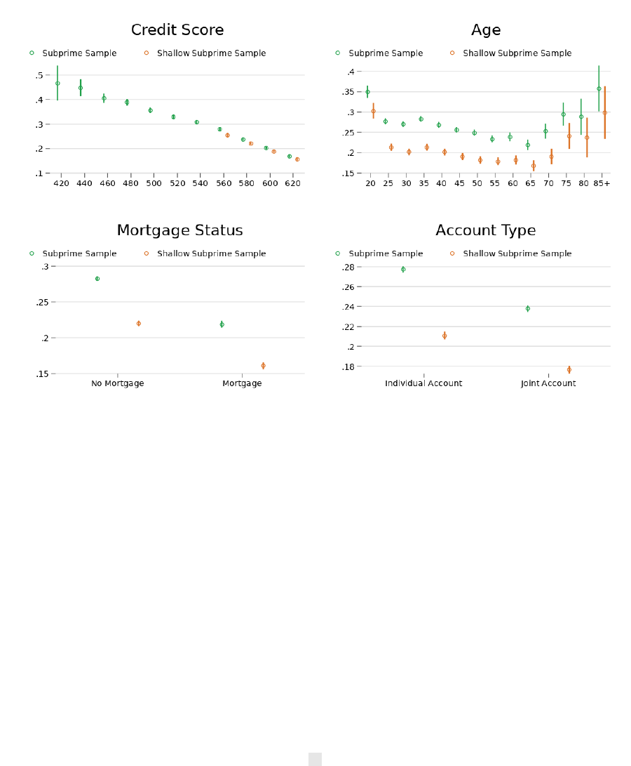
borrowers in our full subprime sample had all the observables they have except for credit scores
at origination of 420. Figure A2 shows that predicted 60+ day delinquency rates are lower for
borrowers with higher credit scores and for borrowers with mortgages, as well for loans with a
co-borrower. The relationship between 60+ day delinquency rates and age is U-shaped, with
the lowest predicted delinquency rates for middle-aged borrowers.
FIGURE A2: 60-DAY+ DELINQUENCY RISK BY OBSERVABLE CHARACTERISTICS
43

APPENDIX C:
Ordinary Least Squares model
details:
Several times in this report, we use observable characteristics of loans and borrowers to predict
the interest rates on actual and hypothetical auto loans. This appendix describes the Ordinary
Least Squares (OLS) model we use to do so. OLS is frequently used in statistical analysis to
predict the probability of continuous variables.
Let R denote the interest rate on an auto loan. We use observable characteristics of the borrower
and the loan in the CCP to predict R. Denote these observable characteristics by
,
…,
. For
example,
may be 1 if a consumer’s loan is from a bank and 0 otherwise,
may be 1 if a
consumer’s loan is from a credit union and 0 otherwise, etc. The OLS regression model assumes
that R is equal to a linear function of the estimated parameters and an unobserved error termε
that is normally distributed with mean zero and standard deviation σ
2
:
=
+ +
+
The parameters
,
…,
are estimated from the data by minimizing the sum of squared
deviations between observed values of R and
+ +
. Once the parameters are
estimated, they provide predicted values of R that are equal to
+ +
. Note that
these predicted values of R can be calculated for any combination of characteristics, whether or
not they actually occur in the data. These predicted values of R are studied in the main body of
the paper.
With the OLS model, the estimated parameter values are easy to interpret. For example, if we
estimate
to be .02, then according to the estimated regression model an increase in
by 1 –
holding everything else constant – predicts an increase in the interest rate R of .02. Figure A3
displays our estimated parameter values for the interest rate regression used to produce Figure
8. Note that, since all the control variables
,
…,
are discrete, all the parameter estimates
are relative to an omitted category. The omitted categories for credit score, age, mortgage
44

status, and account type are, respectively, (1) consumers with a credit score in the 620 bucket
(so 610 or above), (2) consumers in the age 20 bracket (so 22 or younger at loan origination), (3)
consumers without a mortgage, and (4) loans without a co-borrower. For example, Figure A3
shows that our regression predicts that, relative to a consumer with a credit score in the 620
bucket, a consumer with a credit score in the 420 bucket but with the same age, mortgage status,
account type, and lender type would have an interest rate higher by roughly 6%. The regression
predicts that consumers with higher credit scores, with mortgages, and with joint accounts
receive lower interest rates. However, the relationship between borrower age and interest rates
is not strong.
FIGURE A3: ESTIMATED PARAMETER VALUES FOR INTEREST RATE REGRESSION
Figure A4 displays our estimated parameter values for the interest rate regression used to
produce Figure 10. Recall that this regression is identical to that used to produce Figure 8,
except it has controls for lender type interacted with borrower delinquency instead of controls
for lender type. Because of this difference, the estimated parameter values may in theory differ,
so for transparency we show them. In practice, they are virtually identical to the estimated
coefficients from the regression used to produce Figure 8, shown in Figure A3.
45

FIGURE A4: ESTIMATED PARAMETER VALUES FOR INTEREST RATE REGRESSION
46
