multivariable-dvips.dvi

15

Multiple Integration

Consider a surface f(x, y); you might temporarily think of this as representing physical

topography—a hilly landscape, perhaps. What is the average height of the surface (or

average altitude of the landscape) over some region?

As with most such problems, we start by thinking a bout how we might approximate

the answer. Suppose the region is a rectangle, [a, b] × [c, d]. We can di vide the rectangle

into a grid, m subdivisions in one direction and n in the other, as indicated in ﬁgure 15. 1.1.

We pick x values x

0

, x

1

,. . . , x

m−1

in each subdivision in the x direction, and similarly in

the y direction. At each of the points (x

i

, y

j

) in one of the smaller rectangles in the grid,

we compute the height o f the surface: f(x

i

, y

j

). Now the average of these heights should

be (depending on the ﬁneness of t he grid) close to the average height of the surface:

f(x

0

, y

0

) + f(x

1

, y

0

) + ··· + f(x

0

, y

1

) + f(x

1

, y

1

) + ···+ f(x

m−1

, y

n−1

)

mn

.

As both m and n go to inﬁnity, we expect this approxim a tion to converge to a ﬁxed

value, the actual average height of the surface. For reasonably nice functions this does

indeed happen.

385

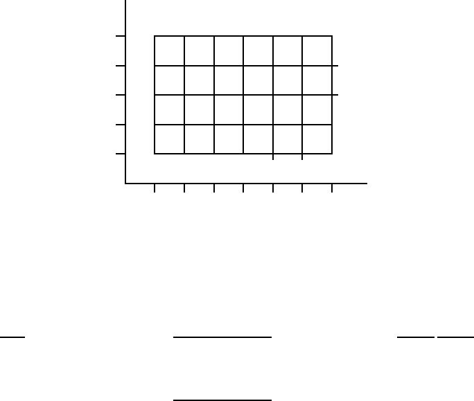
386 Chapter 15 Multiple Integration

c

y

1

y

2

y

3

d

a x

1

x

2

x

3

x

4

x

5

b

∆x

∆y

Figure 15.1.1 A rectangular subdivision of [a, b] × [c, d].

Using sigma notation, we can rewrite the a pproximation:

1

mn

n−1

X

i=0

m−1

X

j=0

f(x

j

, y

i

) =

1

(b − a)(d − c)

n−1

X

i=0

m−1

X

j=0

f(x

j

, y

i

)

b − a

m

d − c

n

=

1

(b − a)(d − c)

n−1

X

i=0

m−1

X

j=0

f(x

j

, y

i

)∆x∆y.

The two parts of this product have useful meaning: (b − a)(d − c) is of course the area of

the rectangle, and the double sum adds up mn terms of the form f(x

j

, y

i

)∆x∆y, which is

the height of the surface a t a point times the a rea of one of the small rectangles into which

we have divided the large rectangle. In short, each term f(x

j

, y

i

)∆x∆y is the volume of a

tall, thin, rectangular box, and is approximately the volume under the surface and above

one of the small recta ngles; see ﬁgure 15.1.2. When we add all of these up, we get an

approximat ion to the volume under the surface and above the rectangle R = [a, b] ×[c, d].

When we take t he limit as m and n go to inﬁnity, the double sum becomes the actual

volume under the surface, which we divide by (b − a)(d − c) to get the average height.

Double sums like this come up in many applications, so in a way it is the most impor-

tant part of this example; dividing by (b − a)(d − c) is a simple extra step that allows the

computation of an average. As we did in the single variable case, we introduce a special

notation for the limit of such a double sum:

lim

m,n→∞

n−1

X

i=0

m−1

X

j=0

f(x

j

, y

i

)∆x∆y =

ZZ

R

f(x, y) dx dy =

ZZ

R

f(x, y) dA,

the double integral of f over the region R. The notati o n dA indicat es a small bit of

area, without specifying any particula r order for the variables x and y; it is shorter and

15.1 Volume and Average Height 387

Figure 15.1.2 Approximating the volume under a surface.

more “generic” than writing dx dy. The average height of the surface in this notatio n is

1

(b − a)(d − c)

ZZ

R

f(x, y) dA.

The next question, of course, is: How do we compute these double integra ls? You

might think that we will need some two-dimensional version of the Fundamental Theorem

of Ca lculus, but a s it turns out we can get away with just the single variable version,

applied twice.

Going back to the double sum, we can rewrite it to emphasize a particula r order in

which we want to add the terms:

n−1

X

i=0





m−1

X

j=0

f(x

j

, y

i

)∆x





∆y.

In the sum in parentheses, only the value of x

j

is changing; y

i

is temporarily constant. As

m goes to inﬁnity, this sum has the right form to turn into an integral:

lim

m→∞

m−1

X

j=0

f(x

j

, y

i

)∆x =

Z

b

a

f(x, y

i

) dx .

So after we take the limit as m goes to inﬁnity, the sum is

n−1

X

i=0

Z

b

a

f(x, y

i

) dx

!

∆y.

388 Chapter 15 Multiple Integration

Of course, for diﬀerent values of y

i

this integral has diﬀerent values; in other words, it is

really a function applied to y

i

:

G(y) =

Z

b

a

f(x, y) dx.

If we substitute back into the sum we get

n−1

X

i=0

G(y

i

)∆y.

This sum has a nice interpretation. The value G(y

i

) is the area of a cross section of the

region under the surface f(x, y) , namely, when y = y

i

. The q uantity G( y

i

)∆y can be

interpreted as the vol ume of a solid with face area G(y

i

) and thickness ∆y. Think of t he

surface f(x, y) as the top of a lo af of sliced bread. Each sli ce has a cross-sectional a r ea and

a thickness; G(y

i

)∆y corresponds to the volume of a single slice of bread. Adding these

up approx imates the total volume o f the loa f. (This is very similar to t he technique we

used to compute volumes in section 9.3, except that there we need the cross-sections to b e

in some way “the same”.) Figure 15.1.3 shows this “sliced loa f” approximation using the

same surface as shown in ﬁgure 15.1.2. Nicely enough, this sum l ooks just like the sort of

sum that turns into an i ntegral, namely,

lim

n→∞

n−1

X

i=0

G(y

i

)∆y =

Z

d

c

G(y) dy

=

Z

d

c

Z

b

a

f(x , y) dx dy.

Let’s be clear about what this means: we ﬁrst will compute the inner integral, temporarily

treating y as a constant. We will do this by ﬁnding an anti-derivative with respect to

x, then substituting x = a and x = b and subtracting, as usual. The result will be an

expression wi th no x variable but some occurrences of y. Then the outer integral will be

an ordinary one-variable problem, with y as the variabl e.

EXAMPLE 15.1.1 Figure 15.1.2 shows the function sin(xy)+6/5 on [0.5, 3.5]×[0.5, 2.5].

The volume under thi s surface is

Z

2.5

0.5

Z

3.5

0.5

sin(xy) +

6

5

dx dy.

The inner integra l is

Z

3.5

0.5

sin(xy) +

6

5

dx =

−cos( x y)

y

+

6x

5



3.5

0.5

=

−cos(3.5y)

y

+

cos(0.5y)

y

+

18

5

.

Unfortunately, this gives a function for which we can’t ﬁnd a simple a nti-derivative. To

complete the problem we could use Sage or similar software to approximate the integral.

15.1 Volume and Average Height 389

Figure 15.1.3 Approximating the volume under a surface with slices. (AP)

Doing this gives a volume of approximately 8.84, so the average height is approximately

8.84/6 ≈ 1.47.

Because a ddition and multiplication are commutative and associative, we can rewrite

the original double sum:

n−1

X

i=0

m−1

X

j=0

f(x

j

, y

i

)∆x∆y =

m−1

X

j=0

n−1

X

i=0

f(x

j

, y

i

)∆y∆x.

Now if we repeat the development above, the inner sum turns int o an integral:

lim

n→∞

n−1

X

i=0

f(x

j

, y

i

)∆y =

Z

d

c

f(x

j

, y) dy,

and then t he outer sum turns into an integral:

lim

m→∞

m−1

X

j=0

Z

d

c

f(x

j

, y) dy

!

∆x =

Z

b

a

Z

d

c

f(x , y) dy dx.

In other words, we can compute the integrals i n either order, ﬁrst with respect to x then

y, or vice versa. Thinking of the loaf o f bread, this corresponds to slicing the loaf in a

direction perpendicular to the ﬁrst.

We haven’t reall y proved that the value of a double integral is equal to the value o f the

corresponding two single integrals in either order of integration, but provi ded the function

is reasonably nice, this is true; the result is called Fubini’s Theorem.

390 Chapter 15 Multiple Integration

EXAMPLE 15.1.2 We compute

ZZ

R

1 + (x −1)

2

+ 4y

2

dA, where R = [0, 3] ×[0, 2], in

two ways.

First,

Z

3

0

Z

2

0

1 + (x − 1)

2

+ 4y

2

dy dx =

Z

3

0

y + (x − 1)

2

y +

4

3

y

3



2

0

dx

=

Z

3

0

2 + 2(x − 1)

2

+

32

3

dx

= 2x +

2

3

(x − 1 )

3

+

32

3

x



3

0

= 6 +

2

3

· 8 +

32

3

· 3 − (0 − 1 ·

2

3

+ 0)

= 44.

In the other order:

Z

2

0

Z

3

0

1 + (x − 1)

2

+ 4y

2

dx dy =

Z

2

0

x +

(x − 1)

3

+ 4y

2

x



3

0

dy

=

Z

2

0

3 +

8

3

+ 12y

2

+

1

3

dy

= 3y +

8

3

y + 4y

3

+

1

3

y



2

0

= 6 +

16

3

+ 32 +

2

3

= 44.

In this example there is no particular reason to favor one direction over the other;

in some cases, one direction might be much easier than the ot her, so it’s usually worth

considering the two diﬀerent possibilities.

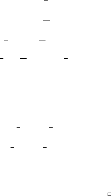
Frequently we wil l be interested in a region that is not simply a rectangle. Let’s

compute the volume under the surface x + 2y

2

above t he region described by 0 ≤ x ≤ 1

and 0 ≤ y ≤ x

2

, shown in ﬁgure 15.1.4.

In principle there is nothing more diﬃcult about thi s problem. If we imagine the three-

dimensional region under the surface and above the para bolic region as an oddly shaped

loaf o f bread, we can still slice it up, approximate the volume of each slice, and add these

15.1 Volume and Average Height 391

0 1

0

1

Figure 15.1.4 A parabolic region of inte gration.

volumes up. For example, if we slice perpendicular to the x axis at x

i

, the thickness of a

slice wi ll be ∆x and the area of the slice will be

Z

x

2

i

0

x

i

+ 2y

2

dy.

When we add these up and take the limit a s ∆x goes to 0, we get the double int egral

Z

1

0

Z

x

2

0

x + 2y

2

dy dx =

Z

1

0

xy +

2

3

y

3



x

2

0

dx

=

Z

1

0

x

3

+

2

3

x

6

dx

=

x

4

+

2

21

x

7



1

0

=

1

4

+

2

21

=

29

84

.

We could just as well slice the solid perpendicular to the y axis, in which case we get

Z

1

0

Z

1

√

y

x + 2y

2

dx dy =

Z

1

0

x

2

+ 2y

2

x



1

√

y

dy

=

Z

1

0

1

2

+ 2y

2

−

y

2

− 2y

2

√

y dy

=

y

2

+

2

3

y

3

−

y

2

4

−

4

7

y

7/2



1

0

=

1

2

+

2

3

−

1

4

−

4

7

=

29

84

.

What is t he average height of the surface over this region? As before, it is the volume

divided by the area of the base, but now we need to use integration to compute the area

392 Chapter 15 Multiple Integration

of the base, since it is not a simple rectangle. The area is

Z

1

0

x

2

dx =

1

3

,

so the average height is 29/28.

EXAMPLE 15.1.3 Find the volume under the surface z =

p

1 − x

2

and a bove the

triangle formed by y = x, x = 1, and the x-axis.

Let’s consider the two possible ways to set this up:

Z

1

0

Z

x

0

p

1 − x

2

dy dx or

Z

1

0

Z

1

y

p

1 − x

2

dx dy.

Which appears easier? In the ﬁrst, the inner integral is easy, because we need an anti -

derivative with respect to y, and the entire i ntegrand

p

1 − x

2

is constant with respect to

y. Of course, the outer integral may be more diﬃcult. In the second, the inner integral

is mildly unpleasant— a t r ig substitution. So let’s try the ﬁrst one, since the ﬁrst step is

easy, and see where that leaves us.

Z

1

0

Z

x

0

p

1 − x

2

dy dx =

Z

1

0

y

p

1 − x

2



x

0

dx =

Z

1

0

x

p

1 − x

2

dx.

This is quite easy, since the substitution u = 1 − x

2

works:

Z

x

p

1 − x

2

dx = −

1

2

Z

√

u du = −

1

3

u

3/2

= −

1

3

(1 − x

2

)

3/2

.

Then

Z

1

0

x

p

1 − x

2

dx = −

1

3

(1 − x

2

)

3/2



1

0

=

1

3

.

This is a good example of how the order of integration can aﬀect the complexity of the

problem. In this case it is possible to do the other order, but it is a bit messier. In

some cases one or der may lead to a very diﬃcult or i mpossible integral; it’s usually worth

considering both possibilities before going very far.

15.1 Volume and Average Height 393

Exercises 15.1.

1. Compute

Z

2

0

Z

4

0

1 + x dy dx. ⇒

2. Compute

Z

1

−1

Z

2

0

x + y dy dx. ⇒

3. Compute

Z

2

1

Z

y

0

xy dx dy. ⇒

4. Compute

Z

1

0

Z

√

y

2

/2

dx dy. ⇒

5. Compute

Z

2

1

Z

x

1

x

2

y

2

dy dx. ⇒

6. Compute

Z

1

0

Z

x

2

0

y

e

x

dy dx. ⇒

7. Compute

Z

√

π/2

0

Z

x

2

0

x cos y dy dx. ⇒

8. Compute

Z

π/2

0

Z

cos θ

0

r

2

(cos θ − r) dr dθ. ⇒

9. Compute:

Z

1

0

Z

1

√

y

p

x

3

+ 1 dx dy. ⇒

10. Compute:

Z

1

0

Z

1

y

2

y sin(x

2

) dx dy. ⇒

11. Compute:

Z

1

0

Z

1

x

2

x

p

1 + y

2

dy dx ⇒

12. Compute:

Z

1

0

Z

y

0

2

√

1 − x

2

dx dy ⇒

13. Compute:

Z

1

0

Z

3

3y

e

x

2

dx dy ⇒

14. Compute

Z

1

−1

Z

1−x

2

0

x

2

−

√

y dy dx. ⇒

15. Compute

Z

√

2/2

0

Z

√

1−2x

2

−

√

1−2x

2

x dy dx. ⇒

16. Evaluate

ZZ

x

2

dA over the region in the ﬁrst quadrant bounded by t he hyperbola xy = 16

and the lines y = x, y = 0, and x = 8. ⇒

17. Find the volume below z = 1 − y above the region −1 ≤ x ≤ 1, 0 ≤ y ≤ 1 − x

2

. ⇒

18. Find the volume bounded by z = x

2

+ y

2

and z = 4. ⇒

19. Find the volume in the ﬁrst octant bounded by y

2

= 4 − x and y = 2z. ⇒

20. Find the volume in the ﬁrst octant bounded by y

2

= 4x, 2x + y = 4, z = y, and y = 0. ⇒

394 Chapter 15 Multiple Integration

21. Find the volume in the ﬁrst octant bounded by x + y + z = 9, 2x + 3y = 18, and x + 3y = 9.

⇒

22. Find the volume in the ﬁrst octant bounded by x

2

+ y

2

= a

2

and z = x + y. ⇒

23. Find the volume bounded by 4x

2

+ y

2

= 4z and z = 2. ⇒

24. Find the volume bounded by z = x

2

+ y

2

and z = y. ⇒

25. Find the volume under the surface z = xy above the tri angle with vertices (1, 1, 0), (4, 1, 0),

(1, 2, 0). ⇒

26. Find the volume enclosed by y = x

2

, y = 4, z = x

2

, z = 0. ⇒

27. A swimming pool is circular with a 40 meter diameter. The depth is constant along east-west

lines and increases linearly from 2 meters at the south end to 7 meters at the north end.

Find the volume of the pool. ⇒

28. Find the average value of f(x, y) = e

y

√

x + e

y

on the rectangle with vertices (0, 0), (4, 0),

(4, 1) and (0, 1). ⇒

29. Figure 15.1.5 shows a te mperature map of Colorado. Use the data to esti mate the average

temperature in the state usi ng 4, 16 and 25 subdivisions. Give both an upper and lower

estimate. Why do we like Colorado for this problem? What other state(s) might we li ke?

Figure 15.1.5 Colorado temperatures.

30. Three cylinders of radius 1 intersect at right angles at the origin, as shown in ﬁgure 15.1.6.

Find the volume contained inside all three cylinders. ⇒

31. Prove that if f(x, y) is integrable and if g(x, y) =

Z

x

a

Z

y

b

f(s, t) dt ds then g

xy

= g

yx

=

f(x, y).

32. Reverse the order of integration on each of the following integrals

a.

Z

9

0

Z

√

9−y

0

f(x, y) dx dy

b.

Z

2

1

Z

ln x

0

f(x, y) dy dx

15.2 Double Integrals in Cylindrical Coordinates 395

Figure 15.1.6 Intersection of three cylinders. (AP)

c.

Z

1

0

Z

π/2

arcsin y

f(x, y) dx dy

d.

Z

1

0

Z

4

4x

f(x, y) dy dx

e.

Z

3

0

Z

√

9−y

2

0

f(x, y) dx dy

⇒

33. What are the parallels between Fubini’s Theorem and Clairaut’ s Theorem (14.6.2)?

Suppose we have a surface given in cylindrical coordinates as z = f(r, θ) and we wish to ﬁnd

the integral over some region. We could attempt to translate into rectangular coordinates

and do the integration there, but it is often easier to stay in cylindrical coordinates.

How might we approximate the volume under such a surface in a way that uses cylin-

drical coordinates directly? The basic idea is the same as before: we divide the region into

many small regions, multiply the area of each small regio n by the height of the surface

somewhere in that little regi o n, and add them up. What changes is the shape of the small

regions; in order t o have a nice representati on in terms of r and θ, we use small pieces

of ring-shaped ar eas, as shown in ﬁgure 15.2.1. Each smal l region is roughly rectangular,

except that two sides a r e segments of a circle and the other two sides are not quite parallel.

Near a point (r, θ), the length of either circular arc is about r∆θ and the length of each

straight side is simply ∆r. When ∆r and ∆θ are very small, the region is nearly a rectangle

with area r∆r∆θ , and the volume under the surface is approximately

XX

f(r

i

, θ

j

)r

i

∆r∆θ.

396 Chapter 15 Multiple Integration

In the limit, this turns into a double integral

Z

θ

1

θ

0

Z

r

1

r

0

f(r, θ)r dr dθ.

.

..

.

..

.

..

.

..

.

..

.

..

.

..

.

∆r

r∆θ

Figure 15.2.1 A cylindrical coordinates “grid”.

EXAMPLE 15.2.1 Find the volume under z =

√

4 − r

2

above the quarter circle

bounded by the two axes a nd the circle x

2

+ y

2

= 4 in the ﬁrst quadrant.

In terms of r and θ, this region is described by the restrictio ns 0 ≤ r ≤ 2 and 0 ≤ θ ≤

π/2, so we have

Z

π/2

0

Z

2

0

p

4 − r

2

r dr dθ =

Z

π/2

0

−

1

3

(4 − r

2

)

3/2



2

0

dθ

=

Z

π/2

0

8

3

dθ

=

4π

3

.

The surface is a portion of t he sphere of radius 2 centered at the origin, in fact exactly

one-eighth of the sphere. We know the formula for volume of a sphere is (4/3)πr

3

, so

the volume we have computed is (1/8)(4/3)π2

3

= (4/3)π, in agreement with our answer.

(From another point of view, what we’ve done is prove that the volume of a sphere of

radius 2 is (32/3). If you replace 2 by a a nd do the integral again, it is not any more

diﬃcult, and you will prove that the volume of a sphere of radius a is (4/3)πa

3

.)

15.2 Double Integrals in Cylindrical Coordinates 397

This exampl e is much like a simple one in rectangular coordinates: the region of

interest may be described exactly by a constant range for each of the variables. As with

rectangular coordinates, we can adapt the method to deal with more complicated regions.

EXAMPLE 15.2.2 Find the volume under z =

√

4 − r

2

above the region enclosed by

the curve r = 2 cos θ, −π/2 ≤ θ ≤ π/2; see ﬁgure 15.2.2. The region is described in polar

coordinates by the inequalities −π/2 ≤ θ ≤ π/2 and 0 ≤ r ≤ 2 cos θ, so the double integra l

is

Z

π/2

−π/2

Z

2 cos θ

0

p

4 − r

2

r dr dθ = 2

Z

π/2

0

Z

2 cos θ

0

p

4 − r

2

r dr dθ.

We can rewrite the integral as shown because of the symmetry of the volume; this avoids

a complicat ion during the evaluation. Proceeding:

2

Z

π/2

0

Z

2 cos θ

0

p

4 − r

2

r dr dθ = 2

Z

π/2

0

−

1

3

(4 − r

2

)

3/2



2 cos θ

0

dθ

= 2

Z

π/2

0

−

8

3

sin

3

θ +

8

3

dθ

= 2



−

8

3

cos

3

θ

3

− cos θ +

8

3

θ





π/2

0

=

8

3

π −

32

9

.

..

.

..

...

....

.......

....

..

.

..

.

..

.

..

...

.........

...

..

.

..

.

Figure 15.2.2 Volume over a region with non-constant limits.

You might have learned a formula for computing areas i n polar coordinates. It i s

possible to compute areas as volumes, so that you need only remember one technique.

398 Chapter 15 Multiple Integration

Consider the surface z = 1, a horizontal pl ane. The volume under this surface and above

a region in the x-y pla ne is simply 1 ·(area of the region), so computing the volume really

just computes the area of the region.

EXAMPLE 15.2.3 Find the area outside the circle r = 2 and i nside r = 4 sin θ; see

ﬁgure 15.2.3. The region is described by π/6 ≤ θ ≤ 5π/6 and 2 ≤ r ≤ 4 sin θ, so the

integral is

Z

5π/6

π/6

Z

4 sin θ

2

1 r dr dθ =

Z

5π/6

π/6

1

2

r

2



4 sin θ

2

dθ

=

Z

5π/6

π/6

8 sin

2

θ − 2 dθ

=

4

3

π + 2

√

3.

Figure 15.2.3 Finding area by computing volume.

Exercises 15.2.

1. Find the volume above the x-y plane, under the surface r

2

= 2z, and inside r = 2. ⇒

2. Find the volume inside both r = 1 and r

2

+ z

2

= 4. ⇒

3. Find the volume below z =

√

1 − r

2

and above the top half of the c one z = r. ⇒

4. Find the volume below z = r, above the x-y plane, and i nsi de r = cos θ. ⇒

5. Find the volume below z = r, above the x-y plane, and i nsi de r = 1 + cos θ. ⇒

6. Find the volume between x

2

+ y

2

= z

2

and x

2

+ y

2

= z. ⇒

7. Find the area inside r = 1 + sin θ and outside r = 2 sin θ. ⇒

8. Find the area inside both r = 2 sin θ and r = 2 cos θ. ⇒

9. Find the area inside the four-leaf rose r = cos(2θ) and outside r = 1/2. ⇒

10. Find the area inside the cardioid r = 2( 1 + cos θ) and outside r = 2. ⇒

11. Find the area of one loop of the three-leaf rose r = cos(3θ). ⇒

15.2 Double Integrals in Cylindrical Coordinates 399

12. Compute

Z

3

−3

Z

√

9−x

2

0

sin(x

2

+ y

2

) dy dx by converting to cyl indrical coordinates. ⇒

13. Compute

Z

a

0

Z

0

−

√

a

2

−x

2

x

2

y dy d x by converting to cylindrical c oordinates. ⇒

14. Find the volume under z = y

2

+ x + 2 above the region x

2

+ y

2

≤ 4 ⇒

15. Find the volume between z = x

2

y

3

and z = 1 above the region x

2

+ y

2

≤ 1 ⇒

16. Find the volume inside x

2

+ y

2

= 1 and x

2

+ z

2

= 1. ⇒

17. Find the volume under z = r above r = 3 + cos θ. ⇒

18. Figure 15.2.4 shows the pl ot of r = 1 + 4 sin(5θ).

Figure 15.2.4 r = 1 + 4 sin(5θ)

a. Describe the behavior of the graph in terms of the given equation. Speciﬁcally, explain

maximum and minimum values, numb er of leaves, and the ‘leaves within leaves’.

b. Give an inte gral or integrals to determine the area outside a smaller leaf but inside a

larger leaf.

c. How would changing the value of a in t he equation r = 1 + a cos(5θ) change the relative

sizes of the inner and outer leaves? Focus on values a ≥ 1. (Hint: How would we change

the maximum and minimum values?)

19. Consider the integral

ZZ

D

1

p

x

2

+ y

2

dA, where D is the unit disk centered at the origin.

(This is the same shape described in a diﬀerent way in exercise 13 in section 9.7.) (See the

graph here.)

a. Why might this integral be considered improper?

b. Calculate the value of the integral of the same function 1/

p

x

2

+ y

2

over the annulus

with outer radius 1 and inner radius δ.

c. Obt ain a value for the integral on the whole disk by letting δ approach 0. ⇒

d. For which values λ can we replace the denominator with (x

2

+y

2

)

λ

in the original integral

and still get a ﬁnite value for the improper integral?

400 Chapter 15 Multiple Integration

Using a single integral we were able t o compute the center of mass for a one-dimensional

object wit h variable density, and a two dimensional object with constant density. With a

double int egral we can handle two dimensions and variable density.

Just as before, the coordinates of the center of ma ss are

¯x =

M

y

M

¯y =

M

x

M

,

where M is the total mass, M

y

is the moment around the y-axis, and M

x

is the moment

around the x-axis. (You may want to review t he concepts in section 9.6.)

The key to the computation, just as before, is the approximation of mass. In the two-

dimensional case, we treat density σ as mass per square area, so when density is constant,

mass is (density)(area). If we have a two-dimensional region with varying density given

by σ(x, y), and we divide the region into small subregions with area ∆A, then the mass of

one subregion is approximately σ(x

i

, y

j

)∆A, the total mass is approximately the sum of

many of these, and as usual the sum turns into an integral in the limit :

M =

Z

x

1

x

0

Z

y

1

y

0

σ(x, y) dy dx,

and similarly for computations in cylindrical coordinates. Then as before

M

x

=

Z

x

1

x

0

Z

y

1

y

0

yσ(x, y) dy dx

M

y

=

Z

x

1

x

0

Z

y

1

y

0

xσ(x, y) dy dx.

EXAMPLE 15.3.1 Find the center of mass o f a thin, uniform plate whose shape is

the region between y = cos x and the x-axis between x = −π/2 and x = π/2. Since the

density is constant, we may take σ(x, y) = 1.

It is clear that ¯x = 0, but for practice let’s compute it anyway. First we compute the

mass:

M =

Z

π/2

−π/2

Z

cos x

0

1 dy dx =

Z

π/2

−π/2

cos x dx = sin x|

π/2

−π/2

= 2.

Next,

M

x

=

Z

π/2

−π/2

Z

cos x

0

y dy dx =

Z

π/2

−π/2

1

2

cos

2

x dx =

π

4

.

15.3 Moment and Center of Mass 401

Finally,

M

y

=

Z

π/2

−π/2

Z

cos x

0

x dy dx =

Z

π/2

−π/2

x cos x dx = 0.

So ¯x = 0 as expected, and ¯y = π/4/2 = π/8. This is the same problem as in example 9.6.4;

it may be helpful to compare the two solutions.

EXAMPLE 15.3.2 Find the center of mass of a two-dimensional plate that occupies

the quarter circle x

2

+ y

2

≤ 1 in the ﬁrst quadrant and has density k(x

2

+ y

2

). It seems

clear that because of the symmetry of both the region and the density function (both are

important!), ¯x = ¯y. We’ll do both to check our work.

Jumping right in:

M =

Z

1

0

Z

√

1−x

2

0

k(x

2

+ y

2

) dy dx = k

Z

1

0

x

2

p

1 − x

2

+

(1 − x

2

)

3/2

3

dx.

This int egral is something we can do, but it’s a bit unpleasant. Since everythi ng in sight

is rela ted to a circle, let’s back up and try polar coordinates. Then x

2

+ y

2

= r

2

and

M =

Z

π/2

0

Z

1

0

k(r

2

) r dr dθ = k

Z

π/2

0

r

4



1

0

dθ = k

Z

π/2

0

1

4

dθ = k

π

8

.

Much better. Next, since y = r sin θ,

M

x

= k

Z

π/2

0

Z

1

0

r

4

sin θ dr dθ = k

Z

π/2

0

1

5

sin θ dθ = k −

1

5

cos θ



π/2

0

=

k

5

.

Similarly,

M

y

= k

Z

π/2

0

Z

1

0

r

4

cos θ dr dθ = k

Z

π/2

0

1

5

cos θ dθ = k

1

5

sin θ



π/2

0

=

k

5

.

Finally, ¯x = ¯y =

8

5π

.

Exercises 15.3.

1. Find the center of mass of a two-dimensional plate that occupies the square [ 0, 1] ×[0, 1] and

has density function xy. ⇒

2. Find the center of mass of a two-dimensional plate that occupies the triangle 0 ≤ x ≤ 1,

0 ≤ y ≤ x, and has density function xy. ⇒

3. Find the center of mass of a two-dimensional plate that occupies the upper unit semicircle

centered at (0, 0) and has density functi on y. ⇒

402 Chapter 15 Multiple Integration

4. Find the center of mass of a two-dimensional plate that occupies the upper unit semicircle

centered at (0, 0) and has density functi on x

2

. ⇒

5. Find the center of mass of a two-dimensional plate that occupies the triangle formed by

x = 2, y = x, and y = 2x and has density function 2x. ⇒

6. Find the center of mass of a two-dimensional plate that occupies the triangle formed by

x = 0, y = x, and 2x + y = 6 and has density function x

2

. ⇒

7. Find the c enter of mass of a two-dimensional plate that occupies the region enclosed by the

parabolas x = y

2

, y = x

2

and has density function

√

x. ⇒

8. Find the centroid of the area in the ﬁrst quadrant bounded by x

2

−8y + 4 = 0, x

2

= 4y, and

x = 0. (Recall that the centroid is t he center of mass when the density is 1 everywhere.) ⇒

9. Find the centroid of one loop of the three-leaf rose r = cos(3θ). (Recall that the centroid is

the center of mass when the density is 1 e verywhere, and that the mass in this case is the

same as the area, whi ch was the subject of exercise 11 in section 15.2.) The computations of

the integrals for the moments M

x

and M

y

are elementary but quite long; Sage can help. ⇒

10. Find the center of mass of a two dimensional object that occupies the region 0 ≤ x ≤ π,

0 ≤ y ≤ sin x, with density σ = 1. ⇒

11. A two-dimensional object has shape given by r = 1 + cos θ and density σ(r, θ) = 2 + cos θ.

Set up the three integrals required to compute the center of mass. ⇒

12. A two-dimensional object has shap e given by r = cos θ and density σ(r, θ) = r + 1. Set up

the three integrals required to compute the center of mass. ⇒

13. A two-dimensional object sits inside r = 1 + cos θ and outside r = cos θ, and has density 1

everyw here. Set up the integrals required to compute the center of mass. ⇒

We next seek to compute the area of a surface above ( or below) a region in the x-y plane.

How might we approximate this? We start, as usual, by dividi ng the region i nto a gri d

of small rectangles. We want to approximat e the area of the surface above one of these

small rectangles. The area i s very close to the area of the tangent plane above the small

rectangle. If the tangent plane just happened to be horizontal, of course the area would

simply be the a r ea o f the rectangle. For a typical plane, however, the area is the area of

a parall el ogram, as indicated in ﬁgure 15.4.1. Not e that the area of the parallelogram is

obviously larger the more “tilted” the tangent plane. I n the interactive ﬁgure you can see

that viewed from above the four parallelog rams exactly cover a rectangular region in the

x-y plane.

Now recall a curious fact: the a r ea of a para llelogram can be computed as the cross

product of two vectors (pag e 314). We simply need to acquire two vectors, parallel to

the sides of the parallelogram and with lengths to match. But t hi s is easy: in the x

direction we use the tangent vector we already know, namely h1 , 0, f

x

i and multiply by ∆x

to shrink it to the ri ght size: h∆x, 0, f

x

∆xi. In the y direction we do the same t hi ng and

get h0, ∆y, f

y

∆yi. The cross product of these vectors is hf

x

, f

y

, −1i∆x ∆y with length

15.4 Surface Area 403

Figure 15.4.1 Sm all parallelograms at points of tangency. (AP )

q

f

2

x

+ f

2

y

+ 1 ∆x ∆y, the area of the para llelogram. Now we add t hese up and take the

limit, to produce the integral

Z

x

1

x

0

Z

y

1

y

0

q

f

2

x

+ f

2

y

+ 1 dy dx.

As before, the limits need not be constant.

EXAMPLE 15.4.1 We ﬁnd the area of the hemisphere z =

p

1 − x

2

− y

2

. We compute

the derivati ves

f

x

=

−x

p

1 − x

2

− y

2

f

y

=

−y

p

1 − x

2

− y

2

,

and then t he area is

Z

1

−1

Z

√

1−x

2

−

√

1−x

2

s

x

2

1 − x

2

− y

2

+

y

2

1 − x

2

− y

2

+ 1 dy dx.

This is a bit on the messy side, but we can use polar coordinates:

Z

2π

0

Z

1

0

r

1

1 − r

2

r dr dθ.

This int egra l is improper, since the function is undeﬁned at the l imit 1. We therefore

compute

lim

a→1

−

Z

a

0

r

1

1 − r

2

r dr = lim

a→1

−

p

1 − a

2

+ 1 = 1,

404 Chapter 15 Multiple Integration

using the substitution u = 1 − r

2

. Then the area is

Z

2π

0

1 dθ = 2π.

You may recall that the area of a sphere of radius r is 4πr

2

, so half the area of a unit sphere

is (1/2)4 π = 2π, in agreement with our answer. (Alternately, we can vi ew this calculation

as proving that the formula for the ar ea of a sphere is correct.)

Exercises 15.4.

1. Find the area of the surface of a right circular cone of height h and base radius a . ⇒

2. Find the area of the portion of the plane z = mx inside the cylinder x

2

+ y

2

= a

2

. ⇒

3. Find the area of the portion of the plane x + y + z = 1 in the ﬁrst octant. ⇒

4. Find the area of the upper half of the cone x

2

+ y

2

= z

2

inside the cylinder x

2

+ y

2

−2x = 0.

⇒

5. Find t he area of the upper half of the cone x

2

+ y

2

= z

2

above the interior of one loop of

r = cos(2θ). ⇒

6. Find the area of the upper hemisphere of x

2

+ y

2

+ z

2

= 1 above the interior of one loop of

r = cos(2θ). ⇒

7. The plane ax + by + cz = d cuts a triangle in the ﬁrst octant provided that a, b, c and d are

all posi tive. Fi nd the area of this triangle. ⇒

8. Find the area of the portion of the cone x

2

+ y

2

= 3z

2

lying above the xy plane and insi de

the cylinder x

2

+ y

2

= 4y. ⇒

It will come as no surprise that we can also do triple integrals—integrals over a three-

dimensional region. The simplest applicatio n allows us to compute volumes in an alternate

way.

To approxi mate a volume in three dimensions, we can divide the three-dimensional

region into small rectangular boxes, each ∆x ×∆y ×∆z with volume ∆x∆y∆z. Then we

add them all up and take the limi t, to get an integral :

Z

x

1

x

0

Z

y

1

y

0

Z

z

1

z

0

dz dy dx.

If the limits are constant, we are simpl y computing t he volume of a rectangular box.

EXAMPLE 15.5.1 We use an integral to compute the volume of the box with opposite

corners at (0, 0, 0) and (1, 2, 3).

Z

1

0

Z

2

0

Z

3

0

dz dy dx =

Z

1

0

Z

2

0

z|

3

0

dy dx =

Z

1

0

Z

2

0

3 dy dx =

Z

1

0

3y|

2

0

dx =

Z

1

0

6 dx = 6 .

15.5 Triple Integrals 405

Of course, this is more interesting a nd useful when the limits are not constant.

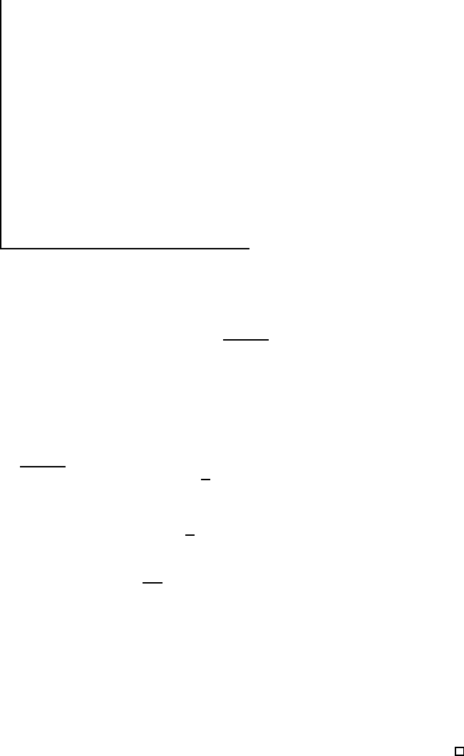
EXAMPLE 15.5.2 Find the volume of the tetrahedron with corners at (0, 0, 0), (0, 3, 0),

(2, 3, 0), and (2, 3, 5).

The whole problem comes down to correctly describing the regi on by i nequalities:

0 ≤ x ≤ 2, 3x/ 2 ≤ y ≤ 3, 0 ≤ z ≤ 5x/2. The lower y limit comes from t he equatio n of

the li ne y = 3x/2 that forms one edge of the tetrahedron in the x-y plane; the upper z

limit comes from the equation of the plane z = 5x/2 that forms the “upper” side of the

tetrahedron; see ﬁgure 15 .5.1. Now the volume is

Z

2

0

Z

3

3x/2

Z

5x/2

0

dz dy dx =

Z

2

0

Z

3

3x/2

z|

5x/2

0

dy dx

=

Z

2

0

Z

3

3x/2

5x

2

dy dx

=

Z

2

0

5x

2

y



3

3x/2

dx

=

Z

2

0

15x

2

−

15x

2

4

dx

=

15x

2

4

−

15x

3

12



2

0

= 15 − 10 = 5.

Pretty much just the way we did for two dimensions we can use triple integration to

compute mass, center of mass, and various average quantities.

EXAMPLE 15.5.3 Suppose the temperature at a point is given by T = xyz. Find the

average temperature in the cube with opposite corners at (0, 0, 0) a nd (2 , 2, 2).

In two dimensions we add up the temperature at “each” point and divide by the area;

here we add up the temperatures and di vide by the volume, 8:

1

8

Z

2

0

Z

2

0

Z

2

0

xyz dz dy dx =

1

8

Z

2

0

Z

2

0

xyz

2



2

0

dy dx =

1

16

Z

2

0

Z

2

0

xy dy dx

=

1

4

Z

2

0

xy

2



2

0

dx =

1

8

Z

2

0

4x dx =

1

2

x

2



2

0

= 1.

406 Chapter 15 Multiple Integration

Figure 15.5.1 A tetrahedron. (AP)

EXAMPLE 15.5.4 Suppose the density of an object is given by xz, and the object

occupies the tetrahedron with corners (0, 0, 0 ), (0, 1, 0), (1, 1, 0), and (0, 1, 1). Find the

mass and center of mass of the object.

As usual, the mass is the integral of density over the region:

M =

Z

1

0

Z

1

x

Z

y−x

0

xz dz dy dx =

Z

1

0

Z

1

x

x(y − x)

2

dy dx =

1

2

Z

1

0

x(1 − x)

3

dx

=

1

6

Z

1

0

x − 3x

2

+ 3x

3

− x

4

dx =

1

120

.

We compute moments as before, except now there is a t hi r d moment:

M

xy

=

Z

1

0

Z

1

x

Z

y−x

0

xz

2

dz dy dx =

1

360

,

M

xz

=

Z

1

0

Z

1

x

Z

y−x

0

xyz dz dy dx =

1

144

,

M

yz

=

Z

1

0

Z

1

x

Z

y−x

0

x

2

z dz dy dx =

1

360

.

Finally, the coordinates of the center of mass are ¯x = M

yz

/M = 1/3, ¯y = M

xz

/M = 5/6,

and ¯z = M

xy

/M = 1/3.

15.6 Cylindrical and Spherical Coordinates 407

Exercises 15.5.

1. Evaluate

Z

1

0

Z

x

0

Z

x+y

0

2x + y − 1 dz dy dx. ⇒

2. Evaluate

Z

2

0

Z

x

2

−1

Z

y

1

xyz dz dy dx. ⇒

3. Evaluate

Z

1

0

Z

x

0

Z

ln y

0

e

x+y+z

dz dy dx. ⇒

4. Evaluate

Z

π/2

0

Z

sin θ

0

Z

r cos θ

0

r

2

dz dr dθ. ⇒

5. Evaluate

Z

π

0

Z

sin θ

0

Z

r sin θ

0

r cos

2

θ dz dr dθ. ⇒

6. Evaluate

Z

1

0

Z

y

2

0

Z

x+y

0

x dz d x dy. ⇒

7. Evaluate

Z

2

1

Z

y

2

y

Z

ln(y+z)

0

e

x

dx dz dy. ⇒

8. Compute

Z

π

0

Z

π/2

0

Z

1

0

z sin x + z cos y dz dy dx. ⇒

9. For each of the integrals in the previous exercises, give a descri pt ion of the volume (both

algebraic and geometric) that is the domain of integration.

10. Compute

Z Z Z

x + y + z dV over the region x

2

+ y

2

+ z

2

≤ 1 i n the ﬁrst octant. ⇒

11. Find the mass of a cube with edge length 2 and density equal to the square of the distance

from one c orner. ⇒

12. Find the mass of a cube with edge length 2 and density equal to the square of the distance

from one edge. ⇒

13. An object occupies the vol ume of the upper hem isphere of x

2

+ y

2

+ z

2

= 4 and has density

z at (x, y, z). Find the center of mass. ⇒

14. An object oc c upies the volume of the pyramid with corners at (1, 1, 0), (1, −1, 0), (−1, −1, 0),

(−1, 1, 0), and (0, 0, 2) and has density x

2

+ y

2

at (x, y, z). Find the center of mass. ⇒

15. Verify the moments M

xy

, M

xz

, and M

yz

of example 15.5.4 by evaluating the integrals.

16. Find the region E for which

ZZZ

E

(1 − x

2

− y

2

− z

2

) dV is a maximum.

We have seen that sometimes double integral s are simpliﬁed by doing them in polar coordi-

nates; not surprisingly, triple integrals are sometimes simpler in cyl indrical coordinates or

spherical coordinates. To set up integrals in polar coordinates, we had to understand the

shape and area of a typical small region into which the region of integration was divided.

We need to do the same thing here, for three dimensional regions.

408 Chapter 15 Multiple Integration

The cylindrical coordinate system is the simplest, since it is just the polar coordinate

system plus a z coordinate. A typical small unit of volume is the shape shown in ﬁg-

ure 15.2.1 “fattened up” in the z direction, so its volume is r∆r∆θ∆z, or in the limit,

r dr dθ dz.

EXAMPLE 15.6.1 Find the volume under z =

√

4 − r

2

above the quarter circle inside

x

2

+ y

2

= 4 in the ﬁrst quadrant.

We could of course do this with a double integra l, but we’ll use a triple int egra l:

Z

π/2

0

Z

2

0

Z

√

4−r

2

0

r dz dr dθ =

Z

π/2

0

Z

2

0

p

4 − r

2

r dr dθ =

4π

3

.

Compare this to example 15.2.1.

EXAMPLE 15.6.2 An object occupies the space inside both the cylinder x

2

+ y

2

= 1

and the sphere x

2

+ y

2

+ z

2

= 4, and has density x

2

at (x, y, z). Find the total mass.

We set this up in cylindrical coordinates, recalling that x = r cos θ:

Z

2π

0

Z

1

0

Z

√

4−r

2

−

√

4−r

2

r

3

cos

2

(θ) dz dr dθ =

Z

2π

0

Z

1

0

2

p

4 − r

2

r

3

cos

2

(θ) dr dθ

=

Z

2π

0



128

15

−

22

5

√

3



cos

2

(θ) dθ

=



128

15

−

22

5

√

3



π

Spherical coordinates are somewhat more diﬃcult to understand. The small volume

we want will be deﬁned by ∆ρ , ∆φ, and ∆θ, as pictured in ﬁgure 15. 6.1. To gain a better

understanding, see the Java applet. The small vol ume is nearly box shaped, with 4 ﬂat

sides and two sides formed from bits o f concentric spheres. When ∆ρ, ∆φ, and ∆θ are all

very small, the volume of this little region will be nearly the volume we get by treating it

as a box. One dimension of the box is simply ∆ρ , the change in distance from the origin.

The other two dimensions are t he lengths of small circular arcs, so they are r∆α for some

suitable r and α, just as in the polar coordinates case.

The easiest of these to understand is the arc corresponding to a change i n φ, which

is nearly identical to the derivation for polar coordinates, as shown in the left graph in

ﬁgure 15.6.2. In that graph we are looking “face on” at the side of the box we are interested

in, so the small angle pictured is precisely ∆φ, the vertical axis really is the z axis, but the

horizontal axis is not a real axis—it is just some line t hrough the origin in the x-y plane.

15.6 Cylindrical and Spherical Coordinates 409

Figure 15.6.1 A small uni t of volume for spherical coordinates. ( AP)

.

..

.

←−−−−−− ρ sin φ −−−−−−→

.

z

∆ρ

ρ∆φ

∆φ

.

..

.

x

y

ρ sin φ∆θ

∆θ

Figure 15.6.2 Setting up integration in spherical coordinates.

Because the other a r c is governed by θ, we need to imag ine looking straight down the z

axis, so that the apparent angle we see is ∆θ. In this view, the axes really are the x and y

axes. In this graph, the apparent distance from the o r igin is not ρ but ρ sin φ, as indicated

in the left graph.

The upshot is that the volume of the little box is approximately ∆ρ(ρ∆φ)(ρ sin φ∆θ) =

ρ

2

sin φ∆ρ∆φ∆θ, or in the limit ρ

2

sin φ dρ dφ dθ.

EXAMPLE 15.6.3 Suppose the temperature a t (x, y, z) is T = 1/(1 + x

2

+ y

2

+ z

2

).

Find the average temperature in the unit sphere centered at the origin.

410 Chapter 15 Multiple Integration

In two dimensions we add up the temperature at “each” point and divide by the area;

here we add up the temperatures and di vide by the volume, (4/3)π:

3

4π

Z

1

−1

Z

√

1−x

2

−

√

1−x

2

Z

√

1−x

2

−y

2

−

√

1−x

2

−y

2

1

1 + x

2

+ y

2

+ z

2

dz dy dx

This looks quite messy; since everything in the probl em is closely related to a sphere, we’ll

convert to spherical coordinates.

3

4π

Z

2π

0

Z

π

0

Z

1

0

1

1 + ρ

2

ρ

2

sin φ dρ dφ dθ =

3

4π

(4π −π

2

) = 3 −

3π

4

.

Exercises 15.6.

1. Evaluate

Z

1

0

Z

x

0

Z

√

x

2

+y

2

0

(x

2

+ y

2

)

3/2

x

2

+ y

2

+ z

2

dz dy dx. ⇒

2. Evaluate

Z

1

−1

Z

√

1−x

2

0

Z

√

2−x

2

−y

2

√

x

2

+y

2

p

x

2

+ y

2

+ z

2

dz dy dx. ⇒

3. Evaluate

Z Z Z

x

2

dV over t he interior of the cylinder x

2

+y

2

= 1 between z = 0 and z = 5.

⇒

4. Evaluate

Z Z Z

xy dV over the interior of the cylinder x

2

+y

2

= 1 between z = 0 and z = 5.

⇒

5. Evaluate

Z Z Z

z dV over the region above the x-y plane, inside x

2

+ y

2

−2x = 0 and under

x

2

+ y

2

+ z

2

= 4. ⇒

6. Evaluate

Z Z Z

yz dV over the region in the ﬁrst octant, inside x

2

+ y

2

−2x = 0 and under

x

2

+ y

2

+ z

2

= 4. ⇒

7. Evaluate

Z Z Z

x

2

+ y

2

dV over the interior of x

2

+ y

2

+ z

2

= 4. ⇒

8. Evaluate

Z Z Z

p

x

2

+ y

2

dV over the interior of x

2

+ y

2

+ z

2

= 4. ⇒

9. Compute

Z Z Z

x + y + z dV over the region inside x

2

+ y

2

+ z

2

= 1 in the ﬁrst octant. ⇒

10. Find the mass of a right c ircular cone of height h and base radius a if t he density is propor-

tional to the distance from the base. ⇒

11. Find the mass of a right c ircular cone of height h and base radius a if t he density is propor-

tional to the distance from its axis of symmetry. ⇒

12. An object occupies the region inside the unit sphere at the origin, and has density equal to

the distance from the x-axis. Find the mass. ⇒

15.7 Change of Variables 411

13. An object occupies the region inside the unit sphere at the origin, and has density equal to

the square of the distance from the origin. Find the mass. ⇒

14. An object occupies the region between the unit sphere at the origin and a sphere of radius

2 with center at the origin, and has density equal to the distance from t he origin. Find the

mass. ⇒

15. An object occupies the region in the ﬁrst octant bounded by the cones φ = π/4 and φ =

arctan 2, and the sphere ρ =

√

6, and has density proportional to the distance from the

origin. Find the mass. ⇒

One of the most useful techniques for evaluating integra ls is substitution, both “u-substitu-

tion” and trigonometric substitution, in which we change the variable to something more

convenient. As we have seen, sometimes changing from recta ngular coordinates to another

coordinate system is helpful, and thi s too changes the variables. This is certainly a more

complicated change, since instead of changing one variable for another we change an entire

suite of variables, but as it turns o ut it is really very similar to the ki nds of change of

varia bl es we al ready know as substitution.

x

0 0.5 1

0

0.1

0.2

0.3

0.4

0.5

u

0 0.5 1 1.5

0

0.1

0.2

0.3

0.4

0.5

Figure 15.7.1 Single change of variable.

Let’s examine the single var iable case again, from a slightly diﬀerent perspective than

we have previously used. Suppose we start with the problem

Z

1

0

x

2

p

1 − x

2

dx;

this computes the area in the left graph of ﬁgure 1 5.7.1. We use the substitution x = sin u

to transform the function from x

2

√

1 − x

2

to sin

2

u

p

1 − sin

2

u, and we also convert dx to

cos u du. Finally, we convert t he limits 0 and 1 to 0 and π/2. This transforms the integral:

Z

1

0

x

2

p

1 − x

2

dx =

Z

π/2

0

sin

2

u

p

1 − sin

2

u cos u du.

We want to notice that there are three diﬀerent conversions: the main function, the diﬀer-

ential dx, and the int erval of integra tion. The function is converted to sin

2

u

p

1 − sin

2

u,

412 Chapter 15 Multiple Integration

shown in the right-hand graph of ﬁgure 15 .7.1. It is evident that the two curves pictured

there have the same y-values in the same order, but the horizontal scale has been changed.

Even though the heights are the same, the two integrals

Z

1

0

x

2

p

1 − x

2

dx and

Z

π/2

0

sin

2

u

p

1 − sin

2

u du

are not the same; clearly the right hand area is la rger. One way to understand the prob-

lem is to note that if both areas are approximated using, say, ten subintervals, that the

approximat ing rectangles on the right are wider than their counterparts o n the left, as in-

dicated. In the picture, the width of the rectangle on the left is ∆x = 0.1, between 0.7 and

0.8. The rectangle on the right is situated between the corresponding values arcsin(0.7)

and arcsin(0.8 ) so that ∆u = arcsin(0.8) − arcsin(0. 7). To make the widths match, and

the a r eas therefore the same, we can multiply ∆u by a correction factor; in t hi s case the

correction factor i s approximately cos u = cos(ar csin(0.7)), w hi ch we compute when we

convert dx t o cos u du.

Now let’s move to functions of two variables. Suppose we want to convert an integral

Z

x

1

x

0

Z

y

1

y

0

f(x , y) dy dx

to use new varia bl es u and v. In the single variable case, there’s ty pi cally just one reason

to want to change t he variable: to make the function “nicer” so t hat we can ﬁnd an

antiderivative. In the two variable case, there is a second potential reason: the two-

dimensional region over which we need to integrate is somehow unpleasant, a nd we want

the region in terms of u and v to be nicer—to be a rectangle, for example. Ideally, of

course, the new function and the new region will be no worse than the originals, and at

least o ne of them will be better; this doesn’t always pan out.

As before, there are three parts to the conversion: the function itself must be rewritten

in terms of u and v, dy dx must be converted to du dv, and the old region must be converted

to the new region. We will develop the necessary techniq ues by considering a particular

example, and we will use an exam pl e we already know how to do by other means.

Consider

Z

1

−1

Z

√

1−x

2

0

p

x

2

+ y

2

dy dx.

The limits correspond to integra ting over the top half of a circular disk, and we recognize

that the function will simplify in polar coordinates, so we would normally convert to polar

15.7 Change of Variables 413

coordinates:

Z

π

0

Z

1

0

√

r

2

r dr dθ =

π

3

.

But let’s instead approach this as a substituti o n problem, starting with x = r cos θ, y =

r sin θ. This pair of equations describes a function from “r-θ space” t o “x-y space”, and

because it involves familiar concepts, it is not too hard to understand what it does. In

ﬁgure 15.7.2 we have indicated geomet rically a bit about how this function behaves. T he

four dots labeled a–d in the r-θ plane correspond to the three dots in the x-y plane; dots a

and b both go to the origin because r = 0. The horizontal arrow in the r-θ plane has r = 1

everywhere and θ ranges from 0 to π, so the corresponding points x = r cos θ, y = r sin θ

start at (1, 0) and fol low the unit circl e counter-clockwise. Finally, the vertical arrow has

θ = π/4 and r ranges from 0 to 1, so it maps to the stra ight arrow in the x-y plane.

Extrapolating from these few examples, it’s not hard to see that every vertical line in the

r-θ plane is tra nsformed to a line through the origin in the x-y plane, and every horizontal

line in the r-θ plane is transformed to a circle with center at the origin i n the x-y plane.

Since we are interested in integrating over the half-disk in the x-y plane, we will integrate

over the rectangle [0, π] ×[0, 1] in the r-θ plane, because we now see that the points in this

rectangle are sent precisely to the upper half disk by x = r cos θ a nd y = r sin θ.

0

1

π

θ

r

.......................................................................................................................................................................................................................................................................................................................................................................................

..

.

..

.

..

.

..

.

• •

•

a

b

c

d

−1 0 1

x

y

• •

•

a, b

c

d

.

..

.

..

.

..

.

..

....

.............

....

...

..

.

..

.

..

.

..

.

Figure 15.7.2 Double change of variable .

At this point we are two-thirds done with the task : we know the r-θ limits of integra-

tion, and we can easily convert the function to the new variables:

p

x

2

+ y

2

=

p

r

2

cos

2

θ + r

2

sin

2

θ = r

p

cos

2

θ + sin

2

θ = r. (15.7.1)

The ﬁnal, and most diﬃcult, task is to ﬁgure out what replaces dx dy. (Of course, we

actually know the answer, because we are in eﬀect converting to polar coordinates. What

we really want i s a series of steps that gets to that right answer but that will also work for

other substitutions that are not so familiar.)

Let’s take a step back and remember how integration arises from approximation. When

we approximate the integra l in the x-y plane, we are computing the volumes of tal l thin

414 Chapter 15 Multiple Integration

boxes, in this case boxes that are ∆x × ∆y ×

p

x

2

+ y

2

. We are aiming to come up with

an integral in the r-θ plane that looks like this:

Z

π

0

Z

1

0

r(?) dr dθ. (15.7.2)

What we’re missing is exactly the right quantity to replace the “?” so that we get the

correct answer. Of course, this integral is also the result of an approximation, in which we

add up volumes o f boxes that are ∆r × ∆θ × height; the problem is that the height that

will give us the correct answer is not simply r. Or put another way, we can t hi nk of the

correct height as r, but the area of the base ∆r∆θ as being wrong. The height r comes

from equation 15.7.1, which is to say, it is precisely the same as the corresponding height

in the x-y version of the integra l. The problem is that the area of t he base ∆x ×∆y is not

the same as the area o f the base ∆r × ∆θ. We can think of the “?” in the integral as a

correction factor that is needed so that ? dr d θ = dx dy.

So let’s think a bout what that li ttle base ∆r ×∆θ corresponds to. We know that each

bit of horizontal line in the r-θ plane corresponds to a bit of circular arc in the x-y plane,

and each bit o f vertical line i n the r-θ plane corresponds to a bit of “radial line” in the x-y

plane. In ﬁgure 15.7.3 we show a typical rectangle in the r-θ plane and its corresponding

area i n the x-y plane.

0

1

π

θ

r

∆r

∆θ

.

.................................................................

.

................................................................

−1 0 1

x

y

.

Figure 15.7.3 Corresponding areas. (AP)

In this case, the region in the x-y plane is approximately a rectangle with dimensions

∆r × r∆θ, but in general the corner angles will not be right angles, so the region will

typical ly be (almost) a parallelogram. We need to compute the area of this parallelogram.

We know a neat way to do this: compute the length of a certain cross product (page 314).

If we can determine an appropriate two vectors we’ll be nearly done.

Fortunately, we’ve really done this before. The si des of t he region in the x-y plane

are formed by temporarily ﬁxing eit her r or θ and lett ing the ot her var iable range over a

small interval. In ﬁgure 15.7.4, for example, the upper right edge of the region is formed

by ﬁxing θ = 2π/3 and letting r run from 0.5 to 0 .75. In other words, we have a vector

function v( r) = hr cos θ

0

, r sin θ

0

, 0i, and we a re interested in a restricted set of values

15.7 Change of Variables 415

for r. A vector tangent to this path is given by t he derivative v

′

(r) = hcos θ

0

, sin θ

0

, 0i,

and a small tangent vector, with length approximately equal to the side of the region,

is hcos θ

0

, sin θ

0

, 0idr. Likewise, if we ﬁx r = r

0

= 0.5, we get the vector function

w(θ) = hr

0

cos θ, r

0

sin θ, 0i with derivative w

′

(θ) = h−r

0

sin θ, r

0

cos θ, 0i and a small tan-

gent vector h−r

0

sin θ

0

, r

0

cos θ

0

, 0idθ when θ = θ

0

(at the corner we’re focusing on). These

vectors are shown in ﬁgure 15.7.4, wit h the actual region outl ined by a dotted boundary.

Of course, since both ∆r and ∆θ are quite large, the parallelogram is not a particularly

good approximatio n to the true area.

−1 0 1

x

y

.

..

.

..

.

..

.

Figure 15.7.4 The approximating parallelogram.

The area of this parallelog r am is the length of the cross product:

h−r

0

sin θ

0

, r

0

cos θ

0

, 0idθ × hcos θ

0

, sin θ

0

, 0idr =



i j k

−r

0

sin θ

0

r

0

cos θ

0

cos θ

0

sin θ

0



dθ dr

= h0, 0, −r

0

sin

2

θ

0

− r

0

cos

2

θ

0

idθ dr

= h0, 0, −r

0

idθ dr.

The length of this vector is r

0

dr dθ. So in general, for any values of r and θ, the a rea

in the x-y plane correspo nding to a small rectangle anchored at (θ, r) in the r-θ plane is

approximat el y r d r dθ. In other words, “r” replaces the “?” in equat ion 15.7.2.

In general, a substitution will start with equations x = f(u, v) and y = g(u, v). Again,

it will be str a ightforward to convert the function being integra ted. Converting the l imits

will require, as above, a n understanding of just how the functions f and g transform the

u-v plane into the x-y plane. Finally, the small vectors we need t o approximate an area will

be hf

u

, g

u

, 0idu and hf

v

, g

v

, 0idv. The cross product of these is h0, 0, f

u

g

v

− g

u

f

v

idu dv

with lengt h |f

u

g

v

− g

u

f

v

|du dv. The quantity |f

u

g

v

− g

u

f

v

| is usually denoted



∂(x, y)

∂(u, v)



= |f

u

g

v

− g

u

f

v

|

416 Chapter 15 Multiple Integration

and called the Jacobian. Note that this is the absolute value of the two by two determinant



f

u

g

u

f

v

g

v



,

which may be easier to remember. (Confusingly, the matrix, the determinant of the matri x,

and the absolute value of the determinant are all called the Jacobian by various authors.)

Because there are two things to worry about, namely, t he form of the function and

the region of int egration, transformations in two (or more) variables are quite trick y to

discover.

EXAMPLE 15.7.1 Integrate x

2

− xy + y

2

over the region x

2

− xy + y

2

≤ 2.

The equation x

2

− xy + y

2

= 2 describes an ellipse as in ﬁgure 15.7.5 ; t he region of

integration is the interior of the ellipse. We wi ll use the transformation x =

√

2u −

p

2/3v,

y =

√

2u +

p

2/3v. Substituting into the function itself we get

x

2

− xy + y

2

= 2u

2

+ 2v

2

.

The boundary of the ellipse is x

2

− xy + y

2

= 2, so the boundary of the corresponding

region in the u-v plane is 2u

2

+ 2v

2

= 2 or u

2

+ v

2

= 1, the unit circle, so this substitution

makes the region o f integra tion si mpl er.

Next, we compute the Jacobian, using f =

√

2u −

p

2/3v and g =

√

2u +

p

2/3v:

f

u

g

v

− g

u

f

v

=

√

2

p

2/3 +

√

2

p

2/3 =

4

√

3

.

Hence t he new integral is

ZZ

R

(2u

2

+ 2v

2

)

4

√

3

du dv,

where R is the interior of the unit cir cl e. This is stil l not an easy integral, but it is easily

transformed to polar coordinates, and then easily integrated.

x

y

.

..

.

..

.

..

.

..

.

..

.

..

.

..

.

..

.

..

.

..

.

..

.

..

.

..

.

..

.

..

.

..

.

..

.

..

.

..

.

..

.

..

.

..

.

..

.

..

.

..

.

..

.

..

.

..

...

..

.....

......

.....

..

...

.

..

.

..

.

..

.

..

.

..

.

..

.

..

.

..

.

..

.

..

.

..

.

..

.

..

.

..

.

...

..

.....

......

.....

..

...

..

.

..

.

..

.

..

.

..

.

..

.

..

.

..

.

..

.

..

.

..

.

..

.

..

.

..

.

..

.

..

.

..

.

..

.

..

.

..

.

..

.

..

.

..

.

..

.

..

.

..

.

..

.

..

.

..

.

..

.

..

.

Figure 15.7.5 x

2

− xy + y

2

= 2

15.7 Change of Variables 417

There is a si milar change of variables formula for tri pl e integrals, though it is a bit

more diﬃcult to derive. Suppose we use three substitution functions, x = f (u, v, w),

y = g(u, v, w), and z = h(u, v, w). The Jacobian determinant is now

∂(x, y, z)

∂(u, v, w)

=



f

u

g

u

h

u

f

v

g

v

h

v

f

w

g

w

h

w



.

Then t he integral is transformed in a simila r fashion:

Z Z Z

R

F (x, y, z) dV =

Z Z Z

S

F (f(u, v, w), g(u, v, w), h(u, v, w))



∂(x, y, z)

∂(u, v, w)



du dv dw,

where o f course the region S in uvw space corresponds to the region R in xyz space.

Exercises 15.7.

1. Complete example 15.7.1 by converting to polar coordinates and evaluating the integral. ⇒

2. Evaluate

ZZ

xy dx dy over the square with corners (0, 0), (1, 1), (2, 0), and (1, −1) in two

ways: directly, and using x = (u + v)/2, y = (u − v)/2. ⇒

3. Evaluate

ZZ

x

2

+ y

2

dx dy over the square with corners (−1, 0), (0, 1), (1, 0), and (0, −1) in

two ways: directly, and using x = (u + v)/2, y = (u − v)/2. ⇒

4. Evaluate

ZZ

(x + y)e

x−y

dx dy over the triangle with corners (0, 0), (−1, 1), and (1, 1) in two

ways: directly, and using x = (u + v)/2, y = (u − v)/2. ⇒

5. Evaluate

ZZ

y(x−y) dx dy over the parallelogram with corners (0, 0), (3, 3), (7, 3), and (4, 0)

in two ways: directly, and using x = u + v, y = u. ⇒

6. Evaluate

ZZ

p

x

2

+ y

2

dx dy over the triangle with corners (0, 0), (4, 4), and (4, 0) using

x = u, y = uv. ⇒

7. Evaluate

ZZ

y sin(xy) dx dy over the region bounded by xy = 1, xy = 4, y = 1, and y = 4

using x = u/v, y = v. ⇒

8. Evaluate

ZZ

sin(9x

2

+ 4y

2

) dA, over the region in the ﬁrst quadrant bounded by the ellipse

9x

2

+ 4y

2

= 1. ⇒

9. Compute the Jacobian for the substitutions x = ρ sin φ cos θ, y = ρ sin φ sin θ, z = ρ cos φ.

418 Chapter 15 Multiple Integration

10. Evaluate

ZZZ

E

dV where E is the solid enclosed by the ellipsoid

x

2

a

2

+

y

2

b

2

+

z

2

c

2

= 1,

using the transformation x = au, y = bv, and z = cw . ⇒