
Regression for M&V: Reference Guide
Version 3.0
May 2024
Prepared for
Bonneville Power Administration
Prepared by
Facility Energy Solutions
Stillwater Energy
SBW Consulting
Contract Number BPA-2-C-92283

Regression for M&V: Reference Guide
i
B O N N E V I L L E P O W E R A D M I N I S T R A T I O N
Table of Contents
1. Introduction ........................................................................................................1
1.1. Purpose .................................................................................................................. 1
1.2. Protocols Version 3.0 .............................................................................................. 1
1.3. How is M&V Defined? ............................................................................................. 1
1.4. Background ............................................................................................................ 2
2. Overview of Regression ....................................................................................3
2.1. Description .............................................................................................................. 3
2.2. Regression Applicability .......................................................................................... 4
2.3. Advantages of Regression ...................................................................................... 5
2.4. Disadvantages of Regression ................................................................................. 5
2.5. Consider Uncertainty when Choosing to Use Regression Analysis ......................... 6
3. The Regression Process ...................................................................................8
3.1. Step 1 - Identify All Independent Variables ............................................................. 9
3.2. Step 2 - Collect Data ............................................................................................... 9
3.3. Step 3 - Clean the Data ........................................................................................ 10
3.4. Step 4 - Graph the Data ........................................................................................ 12
3.5. Step 5 - Select and Develop Model ....................................................................... 13
3.6. Step 6 - Validate Regression Model ...................................................................... 13
3.7. Step 7 - Analysis of Residuals .............................................................................. 14
4. Models ............................................................................................................ 15
4.1. One Parameter Model (Mean Model) .................................................................... 15
4.2. Two Parameter Model (Simple Regression) .......................................................... 15
4.3. Simple Regression Change-Point Models ............................................................. 16
4.4. Multiple Regression .............................................................................................. 16
4.4.1. Categorical Variables ........................................................................................................ 17
4.5. Uncertainty and Confidence Intervals ................................................................... 19
4.5.1. Uncertainty ........................................................................................................................ 19
4.5.2. Confidence Level and Confidence Interval ........................................................................ 21
4.5.3. Prediction Interval.............................................................................................................. 23
4.5.4. Confidence Levels and Savings Estimates ....................................................................... 23
5. Validating Models ........................................................................................... 25
Regression for M&V: Reference Guide
ii
5.1.
Statistical Tests and Measures for the Model ........................................................ 25
5.1.1. R-Squared (Coefficient of Determination) ......................................................................... 25
5.1.2. Adjusted R-Squared .......................................................................................................... 25
5.1.3. Degrees of Freedom ......................................................................................................... 26
5.1.4. Root Mean Squared Error ................................................................................................. 26
5.1.5. Coefficient of Variation of the Root Mean Squared Error .................................................. 26
5.1.6. Bias ................................................................................................................................... 26
5.1.7. F-Statistic .......................................................................................................................... 28
5.1.8. Using Multiple Regressions - VIFs and Multicollinearity .................................................... 28
5.2. Statistical Tests and Measures for the Model’s Coefficients .................................. 29
5.2.1. Standard Error of the Coefficient (Intercept or Slope) ....................................................... 29
5.2.2. t-Statistic ........................................................................................................................... 29
5.2.3. p-value .............................................................................................................................. 30
5.3. Out-of-Sample Testing .......................................................................................... 30
5.4. Analysis of Residuals ............................................................................................ 31
5.4.1. Approximate Normal Distribution ....................................................................................... 32
5.4.2. Constant Variance ............................................................................................................. 32
5.4.3. Uncorrelated with Independent Variables.......................................................................... 33
5.4.4. Independently Distributed (No Autocorrelation) ................................................................. 34
5.4.5. Other Plots ........................................................................................................................ 35
5.5. Tables of Statistical Measures .............................................................................. 35
6. Example ......................................................................................................... 39
6.1. Use of Monthly Billing Data in a 2-Parameter Model to Evaluate Whether It Will
Make a Satisfactory Baseline ................................................................................ 39
6.2. Background on Heating and Cooling Degree-Days (HDD and CDD) .................... 45
7. Minimum Reporting Requirements ................................................................. 47
8. References and Resources ............................................................................ 48
9. Appendix: Glossary of Statistical Terms ........................................................ 50

Regression for M&V: Reference Guide
1
1. Introduction
1.1. Purpose
Regression for M&V: Reference Guide (Regression Guide) as a complement to the Measurement
and Verification (M&V) protocols used by the Bonneville Power Administration (BPA). It assists
the engineer in conducting regression analysis to control for the effects of changing conditions
(such as weather) on energy consumption.
Originally developed in 2012, this Regression Guide is one of ten M&V documents produced by
BPA to direct M&V activities; an overview of the documents is given in the Measurement and
Verification (M&V) Protocol Selection Guide and Example M&V Plan (Selection Guide).
Chapter 8 of this guide provides full citations (and web locations, where applicable) of documents
referenced and an appendix provides a glossary specific to this guide.
1.2. Protocols Version 3.0
BPA revised the protocols described in this guide in 2024. BPA published the original documents
in 2012 as Version 1.0, which were updated to Version 2.0. The current guides are Version 3.0.
1.3. How is M&V Defined?
BPA’s Implementation Manual (the IM) defines measurement and verification as “the process for
quantifying savings delivered by an energy conservation measure (ECM) to demonstrate how
much energy use was avoided. It enables the savings to be isolated and fairly evaluated.”
1
The IM
describes how M&V fits into the various activities it undertakes to “ensure the reliability of its
energy savings achievements.” The IM also states:
The Power Act specifically calls on BPA to pursue cost-effective energy efficiency that is “reliable
and available at the time it is needed.”
2
[…] Reliability varies by savings type: UES, savings
calculators and custom projects.
3
,
4
Custom projects require site-specific Measurement and
Verification (M&V) to support reliable estimates of savings. For UES measures and Savings
Calculators, measure specification and savings estimates must be RTF approved or BPA-
1
2024-2025 Implementation Manual, BPA, April 1, 2024 at https://www.bpa.gov/-/media/Aep/energy-
efficiency/document-library/24-25-im-april24-update.pdf
2
Power Act language summarized by BPA.
3
UES stands for Unit Energy Savings and is discussed subsequently. In brief, it is a stipulated savings value that
region’s program administrators have agreed to use for measures whose savings do not vary by site (for sites
within a defined population). More specifically UES are specified by either the Regional Technical Forum – RTF
(referred to as “RTF approved”) or unilaterally by BPA (referred to as BPA-Qualified). Similarly, Savings Calculators
are RTF approved or BPA-Qualified.
4
Calculators estimate savings that are a simple function of a single parameter, such as operating hours or run time.

Regression for M&V: Reference Guide
2
Qualified[…]. BPA M&V Protocols
5
direct M&V activities and are the reference documents for
reliable M&V..
6
The Selection Guide includes a flow chart providing a decision tree for selecting the M&V protocol
appropriate to a given custom project and addressing prescriptive projects using UES estimates
and Savings Calculators.
M&V is site-specific and required for stand-alone custom projects. BPA’s customers submit
bundled custom projects (projects of similar measures conducted at multiple facilities) as either an
M&V Custom Program or as an Evaluation Custom Program; the latter requires evaluation rather
than the site-specific M&V that these protocols address.
1.4. Background
BPA contracted with a team led by Facility Energy Solutions to assist the organization in revising
the M&V protocols used to assure reliable energy savings for the custom projects it accepts from
its utility customers. The team conducted a detailed review of the 2018 M&V Protocols and
developed the revised version 3.0 under Contract Number BPA-2-C-92283.
The Facility Energy Solutions team is comprised of:
■
Facility Energy Solutions, led by Lia Webster, PE, CCP, CMVP
■
Stillwater Energy, led by Anne Joiner, CMVP
■
SBW Consulting, led by Santiago Rodríguez-Anderson, PE
BPA’s Todd Amundson, PE, PMVE was project manager for the M&V protocol update work. The
work included gathering feedback from BPA and regional stakeholders, and the team’s own review
to revise and update this 2024 Regression Reference Guide.
5
Protocols include: M&V Protocol Selection Guide; reference guides for sampling, regression, and glossary;
protocols on metering, engineering calculations with verification, energy modeling, existing building
commissioning, and strategic energy management.
6
https://www.bpa.gov/-/media/Aep/energy-efficiency/document-library/24-25-im-april24-update.pdf, page 1.

Regression for M&V: Reference Guide
3
2. Overview of Regression
2.1. Description
Regression is a statistical technique that estimates the dependence of a variable of interest (such
as energy consumption) on one or more independent variables, such as ambient temperature. A
regression model estimates the effects on the dependent variable of changes in a given independent
variable, controlling for the influence of other variables. It is a powerful and flexible technique
that can be used in a variety of ways when measuring and verifying the impact of energy efficiency
projects.
This protocol assumes the use of ordinary least squares (OLS) regression. OLS is the most common
form of regression modeling and the default approach in most software packages. OLS is a
mathematical procedure to solve for the set of coefficients that minimize the sum of the squared
differences between the raw data and the fitted linear trend. There are many other forms of
regression modeling, but they are outside the scope of this protocol.
These guidelines are intended to provide energy engineers and M&V practitioners with a basic
understanding of the relevant statistical measures and assumptions necessary to properly use
regression analysis. The guidelines should be followed whenever the technique is required. While
this is not a comprehensive guide to regression, following the approaches described here should
make most M&V regressions valid for their intended purposes. Please refer to a textbook for more
comprehensive information.
Many sources offer additional information on regression analysis. Resources that may be valuable
references for energy efficiency M&V practitioners engaged in regression modeling include the
following:
■
IPMVP: International Performance Measurement and Verification Protocol: Core
Concepts, 2022
7
■
ASHRAE Guideline 14-2023 – Measurement of Energy, Demand, and Water Savings
8
■
California Commissioning Collaborative’s Guidelines for Verifying Existing Building
Commissioning Project Savings
■
NIST/SEMATECH e-Handbook of Statistical Methods, National Institute of Standards
and Technology available at http://www.itl.nist.gov/div898/handbook/ provides a
general reference for exploratory data analysis and statistical inference. This web-
based handbook includes a detailed table of contents and downloadable PDF files for
off-line reading.
7
See also Uncertainty Assessment for IPMVP, 2019.Available at: https://evo-world.org/en/subscribe-join-en
8
Annex B, Determination of Savings Uncertainty, and Annex D, Regression Techniques, have information very
relevant to regression analysis.

Regression for M&V: Reference Guide
4
2.2. Regression Applicability
Regression estimation is useful when a simple spot measurement is not adequate to establish the
baseline energy use. It is applicable when the energy use affected by the efficiency measure is
correlated to one or more independent variables.
Regression analyses may be used when applying any of the M&V protocols, including:
Verification by Meter-Based Energy Modeling
Verification by Equipment or End-Use Metering
Engineering Calculations with Verification
In M&V, energy usage is typically (and optimally) the dependent variable, whether energy usage
is measured monthly through bills or measured more frequently through meter monitoring. The
regression model attempts to predict the value of the dependent variable based on the values of
independent, or explanatory, variables such as weather data.
Dependent Variable – the outcome or endogenous variable; the variable described by the
model; for M&V, the dependent variable is typically energy use
Independent Variable – an explanatory or exogenous variable; a variable whose variation
explains variation in the outcome variable; for M&V, weather characteristics are often
among the independent variables
Simple Regression – a regression with a single independent variable
Multiple Regression – a regression with two or more independent variables
One of the most common applications of regression in M&V is to understand the factors that
influence monthly utility consumption. The initial step is to establish the baseline dependence of
building energy usage on weather conditions and other independent variables (for example,
occupancy and production) by modeling the period prior to the retrofit that is illustrative of pre-
retrofit usage – the baseline period. Then, post-retrofit independent variables are applied to the
baseline model to estimate the building’s energy use had the energy efficiency improvements not
been made (the counterfactual situation). In M&V, this projection of the baseline energy use into
the post period is typically called the adjusted baseline. Finally, the adjusted baseline (predicted
counterfactual energy use) is compared to the actual post-retrofit energy use and the difference
provides an estimate of energy savings.
9
Note that the technique of energy indexing using the Energy Indexing Approach detailed in
Verification by Meter-Based Energy Modeling is a simple application of the regression guide that
9
Note that this is the general approach followed by most M&V practitioners to estimate energy savings. Economists,
who typically conduct impact evaluations, typically estimate a single model from both baseline and post-retrofit
data, and use a dummy (categorical) variable applied to post-retrofit observations to estimate energy use savings.
The resulting savings estimates are comparable to the approach described here, although not necessarily identical.
Regression for M&V: Reference Guide
5
can be used when energy use is linearly proportional to one normalizing (independent) variable.
There are other constraints upon using energy indexing in lieu of a more generalized approach.
When available, the practitioner can use more granular independent variable data to model energy
with a much smaller time interval than a monthly billing period, such as hourly, daily or weekly
data. These smaller interval data are frequently applicable to IPMVP Options A (Key Parameter(s)
Measurement), B (All Parameter Measurement), and C (Whole Facility), and can also be used to
assist in model calibration for IPMVP Option D (Calibrated Simulation), which are reflected in
BPA’s M&V protocols.
2.3. Advantages of Regression
Regression is a very flexible technique that can be used in conjunction with other M&V methods
to help provide a deeper understanding of how and when energy is used. The ideal case for
regression is when the measurement period captures the full annual variation in the dependent and
independent variables – that is, the full range of operation conditions. If the relationship between
the independent and dependent variables is not expected to change over the range of operating
conditions, then short-term measurements can be extrapolated to annual energy use, even if the
measurement period does not capture the full annual variation.
Regression not only facilitates an estimate of energy savings, but also can provide an estimate of
the uncertainty in savings calculations. Further, a baseline regression model can be used to estimate
how much data is required in the post-retrofit period to keep savings uncertainty below a desired
threshold.
Regression is conceptually simple. Most M&V practitioners have at least a basic familiarity with
regression analysis. Further, usage and weather data – the variables typically needed for a basic
model – usually are readily available.
2.4. Disadvantages of Regression
Although simple in concept, proper use of regression requires a clear understanding of statistical
methods and application guidance, which this document seeks to provide to the M&V practitioner.
The information in this guide should be relevant to most M&V projects, but situations can occur
that require a more detailed understanding of statistical methods. While the basic technique is
straightforward, complications to the site or the data can easily require more advanced techniques
and a more thorough understanding of regression methods than this document can provide.
Regression models require multiple observations on the dependent and independent/explanatory
variables. There are times, however, when explanatory variables are not readily available, or we
only have access to proxies. Explanatory variables omitted from a regression model typically
introduce error. If energy use is not a strong function of the independent variable(s) in the equation,
or if there is large variability in energy use relative to strength of the predictive relationship
(“scatter” in the x-y chart; discussed in Section 3.3 and 3.4), regression analysis generates estimates
that have high uncertainty.

Regression for M&V: Reference Guide
6
2.5. Consider Uncertainty when Choosing to Use
Regression Analysis
The relative precision – or fractional savings uncertainty (FSU) – of an energy savings estimate is
the magnitude of the uncertainty relative to the estimate of annual savings.
10
(Note that the savings
need not be annual – perhaps they are just the savings achieved through the reporting period to
date. The formulas just need to be used accordingly.) If a project is expected to save 300,000 kWh
per year and the uncertainty – or margin of error – is ± 75,000 kWh/year, the relative precision of
the estimate is ± 25%.
The Verification by Meter-Based Energy Modeling Protocol includes guidance for calculating the
expected uncertainty (FSU) using baseline data. The key drivers of uncertainty are:
1. The size of the signal – it is easier to precisely measure large effects than small effects.
Savings uncertainty is not a function of expected savings, but the ability of the model to
explain variation in observed usage.
2. Amount of noise in the data – it is easier to precisely measure effects when much of the
variation in pre-installation energy consumption is explained by known independent
variables like weather or production. Savings from projects in facilities with noisy, or
erratic, load patterns will be more uncertain than projects in facilities with more predictable
load patterns.
3. The frequency of the data – it is easier to precisely measure effects with daily or hourly
energy usage data than with monthly data. However, because autocorrelation distorts the
information coming from traditional statistical calculations, the practitioner using hourly
or sub-hourly data will need to take additional modeling steps to produce unbiased
estimates of uncertainty than is necessary with lower frequency data.
The larger the signal, the less the noise, and the higher the frequency of the data each increase the
likelihood that Energy Modeling will be an appropriate M&V approach.
Required Model Sufficiency
Practitioners should be mindful of the uncertainty (standard error or relative precision) in a model
before selecting a regression-based method. Models with lower levels of uncertainty can identify
lower levels of savings, and confidence in savings will be higher.
11
10
ASHRAE. 2014. ASHRAE Guideline 14-2014 – Measurement of Energy, Demand, and Water Savings. Atlanta,
Ga.: American Society of Heating, Refrigerating and Air-Conditioning Engineers.
https://www.techstreet.com/standards/guideline-14-2014-measurement-of-energy-demand-and-water-
savings?product_id=1888937, sec. B4, p. 88 describes fractional savings uncertainty (FSU).
11
IPMVP Core Concepts, 2022

Regression for M&V: Reference Guide
7
Simple regression models should review the standard error (SE) in the predicted energy use. The
expected savings must be greater than twice the standard error of the model for the use of a model
to be valid.
12
Regressions which include noise from unexplained variations such as whole-building models
should evaluate FSU. If the expected relative precision (or FSU) of a project savings estimate is
greater than ± 50%, an alternative protocol could be more appropriate (see Verification by Meter-
Based Energy Modeling for details). It is common to find uncomfortably high relative precision
estimates for projects expected to save less than 5% of facility energy use. In these cases, using a
different M&V protocol should be considered. Verification by Equipment or End-use Metering
Protocol may be able to isolate the affected end-use(s) within a facility and significantly reduce
the amount of noise in the data being modeled (without changing the size of the expected effect).
12
IBID

Regression for M&V: Reference Guide
8
3. The Regression Process
The regression process can be summarized in seven steps, discussed in detail in the following
sections:
1. Identify all independent variables to be included in the regression model
2. Collect the data
3. Clean the data
4. Graph the data
5. Select and develop the regression model
6. Validate the model
7. Analyze the residuals of the model
13
8. Note that for ordinary linear regression to be an appropriate analysis method, the following
conditions must be met:
1. The modeler should be able to reasonably explain the relationship between the dependent
and independent variable(s) prior to performing any regression analysis.
2. The relationship between the dependent variable and all independent variables in the model
(except for indicator variables)
14
should be approximately linear.
3. The model residuals must follow an approximate Normal distribution with a mean of zero
and a constant variance (a condition termed homoscedasticity).
4. The model residuals model must be uncorrelated with each of the independent variables in
the regression model.
5. The model residuals must be independent. That is, the residual at time must not be
correlated with the residual at time 1 or at any other time period.
9. Condition 2, self-explanatory for linear regression, is nonetheless discussed in slightly
more detail in Section 3.4; conditions 3-5 are discussed in greater detail in Section 3.7 and
Section 5.4.
13
Model residuals are the differences between the actual and predicted values.
14
An indicator variable is a binary variable that indicates the presence or absence of some categorical condition
expected to shift the outcome.
Regression for M&V: Reference Guide
9
3.1. Step 1 - Identify All Independent Variables
To properly identify all independent variables, you should consider the facility and how different
factors play into its energy use. Then, you will compile a list of the variables that are likely to have
an impact on the energy use of the facility or system being modeled. When independent variable
values are not numeric or are not continuous, the data can be separated into several regression
models, rather than including all variables within a single model. For example, separate regression
models may be developed for a food processing facility with distinct on- and off-season production
operating modes, resulting in better estimation of baseline energy usage compared to a single
model.
Developing separate models is just one approach to working with categorical variables, an
approach favored by many M&V practitioners. One can also use binary variables to indicate the
presence or absence of a given condition (that is, to create a category) and apply these binary
variables to develop estimates of either the slope or the intercept, or both, when the given condition
is satisfied. (See Section 4.4.1 for a discussion of the use of categorical variables.)
We advise caution when including many variables. A model should only use the variables that
explain the relationship and not include additional, extraneous information. ASHRAE
Guideline 14, Appendix D, provides additional information on regression estimation with two or
more independent variables (multiple regression).
Some independent variables commonly used in energy regressions are:
Ambient dry bulb temperature (actual or averaged over a time-period such as a day)
Heating degree-days (HDD: See Section 6.2)
Cooling degree-days (CDD: See Section 6.2)
Plant output (number of widgets produced in some period)
Number of occupants in a facility each hour
3.2. Step 2 - Collect Data
Prior to installation of the measure, identify and collect data for a monitoring period that is
representative of the facility, operation, or equipment. This is the baseline period, sometimes
referred to as the tuning or pre-period. To provide accurate predictions, the sample of data used to
estimate a regression model should be representative of the full range of operating conditions. That
is, the baseline monitoring period should be long enough to provide “coverage” of the full range
of operating conditions. For example, when analyzing savings for a weather-sensitive measure, the
baseline period typically includes 12 or 24 months of consumption data so that the relationship
between energy usage and weather can be observed across a full range of annual temperature
conditions.
Using consumption data over a partial year may lead to poor predictions for weather conditions
that were not observed in the baseline period. For example, if the baseline period spans from

Regression for M&V: Reference Guide
10
October to April, the baseline period model will not have coverage of hot summer weather
conditions. Consequently, the model will have to predict out-of-sample to estimate energy usage
on a 95-degree day in July. Predicting out-of-sample refers to predictions that are outside of the
range of the independent variables used in the regression model.
3.3. Step 3 - Clean the Data
It is vital that the collected baseline data accurately represent the operation of the facility or system
before improvements were made. Anomalies in the data can have a large effect on the outcome of
the analysis. Thus, after collecting the baseline data (for the dependent variable of interest and any
relevant independent variables), one should spend some time reviewing and “cleaning” the data.
15
Data cleaning efforts, which should be conducted on both the baseline period data and the reporting
period data, typically include:
Examine data outliers. Identify data points that do not conform to the distribution
observed for most of the data and seek an explanation for their unusual values. Atypical
events that result in outliers include equipment failure, situations resulting in abnormal
facility closures, and malfunctioning of the metering equipment. Truly anomalous data
should be documented and then removed from the data set, as they do not describe the
facility or system.
Make any adjustments related to non-routine events. Non-routine events include
renovations, facility expansion, equipment addition or removal, changes to occupancy type
or schedule, and other one-time only or infrequent events. For a discussion of how to make
non-routine event adjustments, refer to Section 3.1.7 of the Verification by Energy
Modeling Protocol.
Identify and address missing data values. If there are large gaps in the data, seek an
explanation and/or alternative data sources, such as a nearby weather station. If data are
missing for a relatively small set of observations, they should be filled in. The practitioner
can fill in a handful of missing hourly temperature values, for example, via simple
averaging (taking the average of the previous reading and the next reading). A more robust
approach, appropriate for more than a handful of missing observations, is to interpolate the
values via regression modeling (that is, creating a regression model to predict the missing
values).
De-duplicate the data. Utility billing and interval data can be susceptible to duplication.
For example, you might have two records for the hour ending 10:00 AM. Those two records
could be exact duplicates, or they might differ slightly. If possible, determine why the
duplication occurred. Regardless, you will want to eliminate records for the same
15
The timing of data cleaning by engineers and by economists commonly diverges. Economists typically collect and
clean both the baseline and the post-installation data as part of Step 2 and conduct the subsequent steps on the
entire pre- and post-period. Engineers typically collect, clean and model baseline data and then turn to the post-
installation data.
Regression for M&V: Reference Guide
11
timestamp. If the records are indeed exact duplicates, just drop one of the records. If one
record is 0 kW and another has a non-zero value, drop the 0 kW record (assuming an actual
read of 0 kW is atypical). If the two records have the same timestamp but different kW
values, perhaps take the average.
Convert all data sources to a common time zone. If you intend on using weather data in
your analysis, it is critical that the time zone of the weather data matches the time zone of
the consumption/demand data (and any other data used in the analysis). Also, be mindful
of records that could be affected by daylight savings time.
Standardize all measurements to a common time unit. The observation interval must be
consistent across all variables. For example, a regression model using monthly utility bills
as the outcome variable requires that all other variables originally collected as hourly, daily,
or weekly data be converted into monthly data points. In such a case, it is common practice
to average (or, if more appropriate, sum) points of daily data over the course of a month,
yielding synchronized monthly data. When working with monthly data, practitioners are
encouraged to use daily averages rather than monthly sums, as the number of days in each
month varies.
Examine scatterplots of the dependent variable versus each independent variable to
determine if any regression outliers are present. Most commonly, one graphs the
independent variables on the X axis and the dependent variable on the Y axis. A “regression
outlier” is a point in the scatterplot that does not fit the overall trend. Such outliers pull the
estimated regression model in their direction, likely leading to a worse overall fit (and
worse fit statistics like root mean squared error (RMSE) and R
2
, discussed further in
Section 5).
Seek an explanation for the occurrence of any regression outliers and remove them if they are truly
anomalous data points, not representative of operating conditions. As an alternative to removing
the outliers, the practitioner could employ a regression approach that reduces the impact of outliers,
such as one based on the mean absolute error.
Figure 3-1 shows an example of a scatter plot of monthly MWh and the number of widgets
produced per month. Note that there is an overall linear trend, but there is one regression outlier
(in red). Also note that this regression outlier is not necessarily an outlier in terms of monthly
MWh or number of widgets produced – it only stands out when the two variables are compared.
The dotted linear trend line describes the full data set and is pulled in the direction of the outlier.
The solid linear trend line describes the relationship without the regression outlier and does a better
job of capturing the overall linear trend.

Regression for M&V: Reference Guide
12
Figure 3-1: Regression Outlier
3.4. Step 4 - Graph the Data
Though subsumed in the previous step, graphing the data warrants a step of its own, as one of the
key requirements for using a linear regression model concerns the relationship between the
dependent variable and the independent variable(s). For linear regression to be a valid, defensible
approach, a scatter plot between the dependent variable and the independent variable(s) must show
an approximate linear trend. This requirement is the pillar of linear regression modeling.
Practitioners should examine scatter plots between the dependent variable and each of the
independent variables used in the model. As an example, Figure 3-1 illustrates a scatter plot for
the linear relationship between monthly energy consumption and the number of widgets produced
per month (with the dependent variable graphed on the Y axis).
When a scatterplot shows multiple distinct linear trends, it is important to investigate whether those
trends correspond with a data category. Common examples include weekday vs. weekend load
patterns and occupied vs. unoccupied operating hours. Section 3.2.2 of the Verification by Energy
Modeling Protocol includes detailed guidance about using categorical variables in regression
models.
Indicator variables, commonly used in regression analysis, are binary (0, 1) categorical values that
indicate presence or absence of a condition expected to shift the outcome. Note that a scatter plot
between the dependent variable and any indicator variables will not show much of the trend since
the indicator variable takes only one of two values. Still, the use of indicator variables is
encouraged, especially if they make a statistically significant contribution to dependent variable
prediction. The concept of statistical significance is discussed in slightly more detail in Section
5.2.3.
0
50
100
150
200
250
75 125 175 225 275 325 375 425 475 525
Monthly Energy Consumption (MWh)
Widgets Produced
Regression for M&V: Reference Guide
13
3.5. Step 5 - Select and Develop Model
After verifying that the relationship between the dependent variable and the independent
variable(s) is approximately linear, one can begin developing regression models. To create a
baseline equation, perform a regression analysis on the measured variables.
The equation calculated from the regression analysis represents the baseline relationship between
the variables of interest. Figure 4-1 in Section 4.2 shows the data and the model estimated for the
value of the outcome variable as a function of one independent variable – a simple regression.
Frequently, however, more than one independent variable influences the outcome variable. For
example, the electricity used by a chiller system might be affected by variations in outside
temperature, relative humidity, hours of facility use, and number of occupants. To accurately
model cooling energy consumption, we need to include multiple independent variables, creating a
multiple regression model. Subsequent sections provide more detailed explanations of model
development, with examples of multiple regression analysis given in Section 4.4.
3.6. Step 6 - Validate Regression Model
Once you have created as baseline (or pre-post) model, there are statistics you should calculate (or,
more appropriately, have software calculate for you) to assess (1) whether or not your independent
variables make significant contributions to the prediction of your dependent variable, (2) the
goodness-of-fit of your model, and (3) the accuracy of your model. These statistics will be noted
here and discussed in greater detail in later sections.
To assess the significance of contributions made by independent variables, some relevant statistics
are:
F-statistic – Section 5.1.7
t-Statistics – Section 5.2.2
p-values – Section 5.2.3
To assess model goodness-of-fit, some relevant statistics are:
R
2
– Section 5.1.1
Adjusted R
2
– Section 5.1.1
To assess model accuracy, some relevant statistics are:
Root Mean Squared Error (RMSE) – Section 5.1.4
CV(RMSE) Coefficient of Variation of the Root Mean Squared Error – Section 5.1.5
Net Determination Bias – Section 5.1.6
For multiple regression models, it’s also advisable to examine variance inflation factors
(VIFs). VIFs can identify whether or not multicollinearity (which occurs when the
Regression for M&V: Reference Guide
14
independent variables are strongly correlated with each other) is a concern.
Multicollinearity and VIFs are discussed in greater detail in Section 5.1.8.
Another popular approach to testing the accuracy of a regression model is called out-of-
sample testing. This entails splitting your original data set into a training and a testing data
set (the training data set is typically larger). The practitioner uses the training data set to
create the regression model and uses the testing data set to test the accuracy of the model
(that is, compare predicted values to actual values). Out-of-sample testing is commonly
used iteratively via a technique called Monte-Carlo cross-validation. Section 5.3 discusses
out-of-sample testing in greater detail.
3.7. Step 7 - Analysis of Residuals
It is rare for a regression model to make predictions that are correct 100% of the time. There is
generally a difference between the predicted values and the actual, observed values. This
difference is referred to as the residual (where residual = actual value – predicted value). Several
of the key assumptions made when fitting an OLS (linear) model concern the distribution of the
residuals. Namely, the residuals must meet the following conditions:
1. Residuals must follow an approximate Normal distribution with a mean of zero.
2. Residuals must have a constant variance (referred to as homoscedasticity). That is,
residuals should not be larger or smaller as the independent variable(s) increases.
3. Residuals must not be correlated with any of the independent variables or the predicted
values of the dependent variable.
4. Residuals must be independent of each other. In other words, the residual at time t must
not be correlated with the residual at time t – 1 (or any other period). This type of
correlation is referred to as autocorrelation and/or serial correlation.
It is essential for the practitioner to check whether these conditions are met. If these conditions are
violated, then conclusions drawn from the regression model could be incorrect. Performing a
residual analysis can also help to identify any regression outliers that might have been overlooked.
The discussion on residual analysis is continued in Section 5.4. There, the reader can find several
methods for checking the conditions noted above.

Regression for M&V: Reference Guide
15
4. Models
This chapter describes types of linear regression models that are commonly used for M&V.
Spreadsheets and statistical software can create simple and multiple regressions – the models most
commonly used in M&V, as discussed below. These tools can also develop second-order or higher
polynomial functions, logistic regressions, and other types of models, which can be appropriate in
certain circumstances. The M&V practitioner should always graph the data in a scatter chart (Step
4 in the process) to verify the type of curve that best fits the data.
The ASHRAE Inverse Model Toolkit (ASHRAE RP-1050) is a useful tool for automating the
creation of the various model types described below.
4.1. One Parameter Model (Mean Model)
Single parameter (1P), or mean models, estimate the mean of the dependent variable and are the
simplest models described in this guide. They are not really regression models but are included
here for completeness. A mean model would describe energy use that is not related to other
independent variables, such as that of a light that runs continuously.
4.2. Two Parameter Model (Simple Regression)
Two parameter (2P) models are the simple linear regression models with which most M&V
practitioners are familiar. They are appropriate for modeling building energy use that varies
linearly with a single independent variable, such as ambient temperature. In most commercial
buildings, metered whole-building energy use varies linearly with ambient temperature above 75º
F due to changes in cooling energy use.
A linear least squares regression with only two parameters is often called a simple regression. The
equation below is the standard form of a simple regression, illustrated in Figure 4-1 with actual
building data.
■
Simple Regression: Y =
β
1
+
β
2
X
1
where: Y = the value of the dependent variable
β
1
= the parameter that defines the y-intercept (the value of y when x equals zero)
β
2
= the parameter that describes the linear dependence on the independent
variable (slope)
X
1
= the value of the independent variable
(Note that statisticians typically describe this model as
0 11
YX
ββ
= +
. In this text, we use the former
notation, as it is consistent with the common engineering terminology two parameter model.)

Regression for M&V: Reference Guide
16
The following graph is an example of a simple regression.
Figure 4-1: Electrical Demand vs. Ambient Temperature
4.3. Simple Regression Change-Point Models
Some systems are dependent on a variable, but only above or below a certain value. For example,
cooling energy use may be proportional to ambient temperature, yet only above a certain threshold.
When ambient temperature decreases to below the threshold, the cooling energy use does not
continue to decrease, because the fan energy remains constant. In commercial buildings with
economizer cooling, this threshold is often 55º F. Similar behavior is often seen in building gas
usage, because the heating energy is proportional to ambient temperature during the space heating
season and the energy associated with hot water use is constant across all seasons.
In cases like these, simple regression can be improved by using a change-point linear regression.
Change point models often have a better fit than a simple regression, especially when modeling
energy usage for a facility. Because of the physical characteristics of buildings, the data points
have a natural 2-line angled pattern to them, that is, display a linear relationship that changes (has
a different slope) at a given point. Sometimes it is even appropriate to use multiple change points.
The practitioner interested in estimating change-point models should consult BPA’s Verification
by Energy Modeling Protocol, Chapter 3, for a complete discussion of change-point models.
4.4. Multiple Regression
The simple regression and change-point models discussed thus far have all used a single
independent variable. Of course, for many building systems, energy use is dependent on more than
y = 7.4282x - 19.351
R² = 0.7582
0
100
200
300
400
500
600
700
800
40 45 50 55 60 65 70 75 80 85 90
Electrical Demand (kW)
Ambient Temperature (°F)
kW
Base Fit
Regression for M&V: Reference Guide
17
one variable. In such cases, single variable models will typically result in low R
2
values. When
using only one independent variable, the equation has only limited ability to predict the dependent
variable, because it does not account for other key factors that should be present in the model.
In such cases, including other variables that are known to influence energy usage will provide a
more accurate model. Commonly used variables whose variation is related with variation in energy
use include: hours of occupancy in buildings, number of employees on given day, meals served at
a restaurant, amount of conditioned floor space, equipment or appliances in use, and water usage.
Including two or more independent variables produces a multiple regression model.
Simple regression can be visualized as fitting a line. Multiple regression models with two
independent variables fit a plane, and a three-variable model fits a 3-dimensional space. The
general format of the model is.
■
Y = β
1
+ β
2
X
1
+ β
3
X
2
+ β
4
X
3
+ … + β
i
X
i-1
where: i = the number of predictors
Note that in common statistics terminology, multiple regression typically refers to regression
models with two or more independent variables and a single dependent variable. In multivariate
regression, by contrast, there are multiple dependent variables and any number of predictors. The
ASHRAE Inverse Model Toolkit refers to multiple regression models and change-point models with
multiple independent variables as multiple-variable or multi-variable models.
Note that additional independent variables will always improve the model’s fit (as measured by
R
2
) regardless of whether or not those variables help in the prediction of observed usage. However,
this does not necessarily mean that the model is improved. With multiple regression models,
practitioners should refer to adjusted R
2
rather than R
2
. The “adjusted” version of this statistic
essentially attaches a penalty for each additional explanatory variable in the model. See Section
5.1.2 for more discussion on adjusted R
2
.
4.4.1. Categorical Variables
Energy use modeling can account for change of states (broadly, the influence of categorical
variables, defined and discussed in this section) by estimating separate models for each state,
estimating a single model with categorical variables, and estimating change-point models (a
specific form of a model with categorical variables, described in the previous section). Most energy
models for M&V will have only one continuous independent variable but may also incorporate
categorical variables.
Variables can be divided into two general types: continuous and categorical. Continuous variables
are numeric and can have any value within the range encountered in the data. Continuous variables
are either interval or ratio numbers (where a value of 10 is twice the magnitude as a value of 5).
Continuous variables are measured things, such as energy use or ambient temperature. Categorical
variables include things like daytype (weekday or weekend, or day of week), occupancy (occupied
or unoccupied), and equipment status (on or off). As examples, occupancy status is a categorical
variable, while number of occupants is a continuous variable.
Regression for M&V: Reference Guide
18
For use in a regression analysis, any categorical variable must be expressed in a binary form, such
as taking the value of 1 for Monday and taking the value of 0 for all other days. This is because all
the variables in a regression model must be linearly related to the dependent variable. A conceptual
category such as day-of-week therefore cannot be included in a regression if it takes values such
1 for Monday, 2 for Tuesday, on up through 7 for Sunday; Tuesday does not have twice the impact
on the dependent variable than Monday, nor does Wednesday have three times the impact.
As mentioned at the end of the prior section, one needs to take care in adding additional variables
– such as multiple binary variables to describe a composite concept (such as day-of-week) –
because the model can become over-specified, and the parameter estimates inaccurate and
imprecise. Thus, when needing to create a set of binary variables to capture a composite categorical
concept, the M&V practitioner should consider the most concise way to express the underlying
relationships between these categories and the dependent variable. Continuing with the day of
week example, it may be that activity ramps up during the week; appropriate categories might be
Monday/Tuesday, Wednesday/Thursday/Friday, and Saturday/Sunday, where Mon_Tues has the
value of 1 if the day is a Monday or Tuesday and 0 otherwise, and similarly for the other variables.
Finally, when working with binary variables describing composite categories, the modeler includes
one less binary variable in the equation than the total number of categories in the set. Continuing
with the example, when the variables Mon_Tues and Wed_Thus_Fri both have the value of 0, the
day must be a Saturday or Sunday; it would be redundant (that is collinear) to add the variable
Sat_Sun.
According to ASHRAE RP-1050, practitioners using categorical variables commonly err by
inappropriately using them only to change the line’s intercept. The M&V practitioner needs to
carefully consider whether the categorical variable is expected to affect the model’s intercept term,
a slope term, or both. If the slope likely differs among categories, the model must include terms to
capture the interaction of the categorical and continuous variable, which can be tedious and error-
prone to accomplish in Microsoft Excel. (Another solution is to fit separate models for different
levels of the categorical variable.)
An appropriate statistical approach to apply with categorical variables is the General Linear Model
(GLM). Multiple regression is typically used where the independent variables are continuous, but
a general linear model can accommodate both categorical and continuous predictor variables. In
avoiding the common pitfall of all categories having the same slope, it is important to use the
proper GLM method. (Please refer to a statistics text for further discussion of general linear
models. Some resources are noted in the References and Resources section of this document.)
Instead of using a multiple regression of the format in ASHRAE RP-1050, you can create separate
models for each category or combination of categories, and then combine these individual models
into a complete model. The basic process is similar to using IF statements to determine, for each
data point, the category of the categorical independent variable, and then using the intercept and
slope that are appropriate for that category.

Regression for M&V: Reference Guide
19
4.5. Uncertainty and Confidence Intervals
4.5.1. Uncertainty
Regression analysis yields estimates, predictions that will not be 100% accurate. Thus, modelers
speak of the uncertainty of the estimates, that is, uncertainty in the predicted y-value. Uncertainty
in regression analysis results from three principal sources:
Measurement uncertainty or measurement error,
Coverage error, and
Regression uncertainty or model uncertainty.
Measurement Uncertainty
Measurement uncertainty has two principal components: measurement bias and measurement
precision. Bias relates to issues of calibration and accuracy; precision relates to the magnitude of
random variation that occurs when multiple measurements are made. Figure 4-2 illustrates these
concepts. The concept of measurement uncertainty as it relates to regression analysis pertains to
the independent variables, as any measurement error in the dependent variable contributes to
model uncertainty, with the error contributing to the model residual.
Figure 4-2: Accuracy vs. Precision
Regression for M&V: Reference Guide
20
Instruments for acquiring measurements should be of sufficient resolution and precision that the
uncertainties in measurements are small relative to the regression uncertainty. Measurement bias
due to measuring equipment error should be eliminated through calibration, and careful
instrumentation design and installation should be used to minimize other measurement bias errors.
Installation criteria for accurate measurement, such as the need for a straight duct of a specific
number of equivalent duct diameters for a flow measurement, may be important.
Note that, even though an installation limitation may introduce the same bias to the pre and post
periods, the fact that the bias is the same may not mean that the savings estimate is not biased.
Whether or not there is a savings bias is dependent upon the type of bias (that is, additive or
multiplicative) and how the measurement is mathematically used.
As applicable and possible, utility meters should be used for energy-use measurements. By M&V
convention, utility meter data is considered to have zero uncertainty for savings estimates.
Similarly, data from a nearby National Oceanic and Atmospheric Administration (NOAA) weather
station should be used for weather measurements, but such measurements should be verified to be
representative of the conditions at the treated building. NOAA sites are far less likely to have
biases or inaccuracies due to solar effects and sensor calibration errors than site measurements.
Specific to weather data, check for evidence of instrumentation changes over time. For example,
one might take differences with nearby weather station data and plot over time. Some stations may
also document such changes. A change in a weather data measurement source during the baseline
or post period may require: (1) the inclusion of an indicator variable for the effected period in the
regression model, (2) a normalization of the weather data, or (3) a full update to the original energy
model.
For a thorough discussion of measurements, refer to Section 6, Instrumentation, and Annex A,
Physical Measurements, within ASHRAE Guideline 14, Measurement of Energy, Demand, and
Water Savings.
Coverage Error
Coverage error occurs when an M&V data set does not fully “cover” the range of conditions that
drive energy use, which is the full range of building or system operating conditions. As stated in
Section 3.2, measurements should be conducted for a sufficient period to capture a significant
range of the independent variable(s). Beyond that, no definitive criteria can be provided regarding
the sufficiency of shorter-term data for annual extrapolation. ASHRAE Research Project 1404,
Measurement, Modeling, Analysis and Reporting Protocols for Short-term M&V of Whole
Building Energy Performance provides some guidance.
In a production environment, the consistency of production will determine this length of time.
When weather is the independent variable, the season and climate will determine the length of
time necessary. If seasonal variations in weather are minor, a relatively short time may be possible
and still cover a wide range of conditions. If seasonal variations are significant, longer periods (up
to a year) may be advisable.
Measurements of the dependent and independent variables must cover the same time periods.

Regression for M&V: Reference Guide
21
Regression Uncertainty
Regression uncertainty (also referred to as savings uncertainty) results both from modeling errors
– explanatory variables are omitted from the model or an incorrect functional form is specified –
and because people’s unpredictable behaviors affect energy use. Uncertainty in regression
typically refers to the uncertainty in the output from a regression; uncertainty in the regression
coefficients is typically referred to in a more explicit manner as the uncertainty of the slope.
A goal of any M&V plan should be to minimize uncertainty in the savings estimate (regression
uncertainty). More specifically, the goal should be to make the uncertainty small relative to the
savings. ASHRAE Guideline 14-2023, Annex B refers to this as the fractional savings uncertainty
(FSU).
16
Generally, factors that affect regression modeling uncertainty include:
Number of points used in the baseline regression
Number of points in the post-installation period
Number of significant independent variables included in the regression
One way to reduce the fractional savings uncertainty is to use more data. Gathering data over a
longer period, and/or at more frequent intervals, will generally reduce the uncertainty. Note,
though, that as data is gathered at more frequent intervals, this will increase serial autocorrelation
– each reading becomes more significantly related to the prior reading. Uncertainty estimates must
account for this autocorrelation. Costs may be affected by increasing the length of time required
to collect data or monitoring additional variables.
Another way to reduce the fractional savings uncertainty is to include more relevant independent
variables. The t-statistic and p-value should be used to check for the relevance of additional
independent variables.
As with all M&V protocols, the emphasis on accuracy needs to be balanced against the level of
savings and cost. Factors affecting regression uncertainty should be assessed to determine the
amount of effort and cost needed to increase accuracy.
4.5.2. Confidence Level and Confidence Interval
Uncertainty is associated with a given confidence level– for example, “We are 90% confident that
the range 433 and 511 kWh bands the true value,” or, as it is more commonly but less accurately
expressed, “We are 90% confident that the true value lies between 433 and 511 kWh.” Confidence
level is an input number; for a given sample and regression, the higher the confidence level
specified, the larger the estimated range that is likely to contain the true value that proportion of
the time.
16
Refer to ASHRAE Guideline 14-2023, Annex B: Determination of Savings Uncertainty for a more detailed
discussion of savings uncertainty than is provided here.

Regression for M&V: Reference Guide
22
Confidence intervals are a common way to express uncertainty. A 95% confidence level implies
that there is a 95% chance that the confidence interval resulting from a sample contains the true
value. Confidence intervals define the range – an uncertainty band – that is expected to band the
true relationship between the dependent and independent variables, with a certain probability. The
width of the confidence interval provides some idea of uncertainty about the estimated values. For
example, the results of a regression analysis of savings may be reported as “500 kWh ±5% at the
95% confidence level.” This means that there is a 95% chance that the confidence interval of 475
to 525 kWh contains the true value of savings. A statement of “500 kWh ±5% at the 68%
confidence level” means that there is only a 68% chance that the true savings value is between
these limits, and a 32% chance that it is outside them.
The practitioner should note that the true value does not fluctuate; rather, because of regression
uncertainty (and, perhaps, measurement uncertainty), there cannot be complete certainty that the
true savings value lies within these limits. Confidence limits are the bounds of the confidence
interval.
Figure 4-3 provides a graphical representation of confidence intervals. The bounded confidence
intervals in this figure demonstrate that higher chances an interval contains the true regression line
require wider intervals than lower chances (that is, the wider the confidence interval, the more
likely it is to contain the true value). The lines in this figure represent upper and lower confidence
limits.
Figure 4-3: Confidence Intervals for a Regression
0
1
2
3
4
5
6
7
8
20 30 40 50 60 70 80 90 100
Normalized Demand (Watts per Sqare Foot)
Ambient Temperature (ºF)
Data
Upper Confidence Limit, 95% Confidence Level
Lower Confidence Limit, 95% Confidence Level
Upper Confidence Limit, 80% Confidence Level
Lower Confidence Limit, 80% Confidence Level
Linear (Data)
The odds are 80%
that these lines
band the true
relationship.
The odds are
95% that
these lines band
the true relationship.

Regression for M&V: Reference Guide
23
4.5.3. Prediction Interval
Prediction intervals are like confidence intervals, but rather than estimating the distribution of a
true value (such as average demand), prediction intervals provide a range of values within which
a single value is expected to fall. As an example of the distinction, a confidence interval can
provide a range of values within which average demand is expected to fall when the ambient
temperature is 60ºF. A prediction interval can provide a range of values within which observed
demand is expected to fall when the ambient temperature is 60ºF. Prediction intervals are wider
than confidence intervals since, under the identical conditions, it is more difficult to predict the
value of a future point than it is to predict the distribution of the population mean.
Figure 4-4 illustrates prediction intervals, adding them to Figure 4-3, above.
Figure 4-4: Prediction Intervals for a Regression
4.5.4. Confidence Levels and Savings Estimates
Savings estimated from regression analyses should describe the range of values corresponding to
a given confidence level. If a single savings estimate, rather than a range, is required, the savings
estimate should be the mean point estimate (that is, the value that falls directly in the middle of the
confidence interval).
0
1
2
3
4
5
6
7
8
20 30 40 50 60 70 80 90 100
Normalized Demand (Watts per Sqare Foot)
Ambient Temperature (ºF)
Data
Upper Confidence Limit, 95% Confidence Level
Lower Confidence Limit, 95% Confidence Level
Upper Confidence Limit, 80% Confidence Level
Lower Confidence Limit, 80% Confidence Level
Upper Prediction Line, 95% Confidence Level
Lower Prediction Line, 95% Confidence Level
Upper Prediction Line, 80% Confidence Level
Lower Prediction Line, 80% Confidence Level
Linear (Data)
The odds are
80% that these
lines band the
true y values.
The odds are
95% that these
lines band the
true y values.
The odds are 80%
that these lines
band the true
relationship.
The odds are
95% that
these lines band
the true relationship.
Regression for M&V: Reference Guide
24
The less scatter, or variability, in the data, the narrower the confidence intervals; greater scatter
results in winder confidence intervals. However, regardless of the degree of scatter, the confidence
interval will be wider when requiring a higher probability that it contains the true regression line
or the true value of savings than when requiring a lower probability. For example, the interval
estimated for a 99% confidence interval will be wider than it will be for a 95% confidence interval.
For a single value of savings, requiring a greater probability that an interval contains the true value
results in a wider uncertainty band, which in turn results in a lower estimate of minimum likely
savings. If a lower probability is acceptable, the uncertainty band will be narrower and the
estimated minimum savings will be higher. To summarize, the minimum savings estimated is
higher with a lower confidence level and is lower with a higher confidence level.

Regression for M&V: Reference Guide
25
5. Validating Models
5.1. Statistical Tests and Measures for the Model
After developing the regression model, you must assess its goodness of fit. There are many ways
of testing regression models. The following is an engineering layperson’s description of some of
the statistical measures and methods used as guidance for validating models. Interim measures
needed for the statistical tests, such as root mean squared error, are also described in this section.
5.1.1. R-Squared (Coefficient of Determination)
The coefficient of determination (R
2
) provides a measure of how well the independent variables
explain variation in the dependent variable. R
2
values range from 0 (indicating none of the variation
in the dependent variable is associated with variation in any of the independent variables) to 1
(indicating all of the variation in the dependent variable is associated with variation in the
independent variables, a “perfect fit” of the regression line to the data). The rule-of-thumb for an
acceptable model using monthly billing data is an R
2
> 0.75.
If the R
2
is low, you may wish to return to Step 5 in the regressions process (see Chapter 3) and
select additional independent variables that may explain energy use and add them to your model;
then use the adjusted R
2
(see Section 5.1.2) as a goodness-of-fit test for a multiple regression.
The R
2
value can be thought of as a goodness-of-fit test; but a high R
2
value is not enough to say
the selected model fits the data well, nor that a low R
2
indicates a poor model. Professional
judgment should be applied, and other fit criteria in addition to R
2
should be assessed. For
CV(RMSE) (see Section 5.1.5), a low value (often interpreted as 10% or 15%) is desirable. For
example, a model with a low R
2
is acceptable when there is a clear relationship between the
dependent and independent variables, as evidenced by the following: The scatter of the observed
y-values around the regression line is low, yet large in relationship to the total scatter of y-values
from the mean of y, and total y scatter is much smaller than the total scatter of x-values from its
mean (this results in a low slope estimate). In a situation where the total scatter of y and x compared
to their means is more comparable, a low R
2
can be acceptable when the estimated coefficient of x
is significant, despite the unexplained variation; however, there will be relatively high uncertainty
in the resulting savings estimates.
The calculations for estimating uncertainty are described in Section 4.5.
5.1.2. Adjusted R-Squared
In multiple regression models, the addition of an independent variable will always result in an
increase in the model’s R
2
, which means the basic R
2
value is not an appropriate indicator of model
fit. Instead, one should judge model fit using adjusted R
2
, a value produced by adjusting R
2
,
dividing R
2
by the associated degrees of freedom (discussed next). The value of the adjusted R
2
only increases from one model specification to another if the additional independent variable(s)
improve the model more than by random chance.
Regression for M&V: Reference Guide
26
5.1.3. Degrees of Freedom
Degrees of freedom (DF) is a common input for statistical calculations. Degrees of freedom is the
number of values in a calculation that are free to vary and is calculated by subtracting the number
of parameters in the model from the total number of data points.
5.1.4. Root Mean Squared Error
Root mean squared error (RMSE) is an indicator of the scatter, or random variability, in the data,
and hence is an average of how much an actual y-value differs from the predicted y-value. It is the
standard deviation of errors of prediction about the regression line.
5.1.5. Coefficient of Variation of the Root Mean Squared Error
Coefficient of variation of the root mean squared error – CV(RMSE) – is the RMSE normalized
by the average y-value. Normalizing the RMSE makes this a nondimensional that describes how
well the model fits the data. It is not affected by the degree of dependence between the independent
and dependent variables, making it more informative than R-squared for situations where the
dependence is relatively low.
5.1.6. Bias
Bias refers to any systematic differences between actual energy use and that predicted by a
regression model. It can result from many parts of the analysis process, including mis-specified
regression models or a lack of coverage in the independent or dependent variables, among others.
Energy models should always be checked for bias: Does the model accurately re-create the actual
baseline energy use on average? Demand models, on the other hand, generally do not require a
bias check, since demand is not summed over time. Also, demand models will generally not require
different points to have different weights, so that potential for bias error (from not using a weighted
regression when one is warranted) is not a concern. Since regression itself minimizes the error for
each point, there will typically be no need to check bias for a demand model. M&V practitioners
should take care to understand any unique situations that may require checking for bias in a demand
model.
Two indices are defined in ASHRAE Guideline 14 for checking energy model bias. These two
indices are net determination bias error (or mean bias error) and normalized mean bias error. Be
forewarned that the Guideline is somewhat confusing, since these two indices are nearly the same
and the document refers to one of the indices using two different terms.
Net determination bias is simply the percentage error in the energy use predicted by the model
compared to the actual energy use. The sum of the differences between actual and predicted energy
use should be zero. If the net determination bias = 0, then there is no obvious bias. ASHRAE
Guideline 14-2014 accepts an energy model if the net determination bias error is less than 0.005%.
Often, bias may be minor, but it still will affect savings estimates. If the savings are relatively large
compared to the bias, bias may not be important. But in many cases, bias could be influential.

Regression for M&V: Reference Guide
27
■
Net Determination Bias Error (NDBE): NDBE
■
Normalized Mean Bias Error (NMBE):
In the equations above,
represents actual energy usage,
represents predicted energy usage,
, represents average energy usage, represents the dumber of data points, and represents the
number of explanatory variables in the model. Note that the two indices are identical if, in NMBE,
p = 0. Therefore, the only difference between the two bias error calculations is an adjustment for
the number of parameters in the model.
Since there is no averaging occurring, it seems that mean bias error is a misnomer. The net
determination bias error is simply the percentage error in total energy use predicted by the model
over the relevant (baseline) time period. In the equation for normalized mean bias error, there is
an average term in the denominator, but the result is still simply a percent error, which is adjusted
for the number of parameters in the model.
Regression models by themselves will not typically have any bias if created properly. However, as
stated above, there can be bias when using regression models, either because multiple categories
need to be considered, or because an unweighted regression was used when data points should not
have equal weights.
Checking for model bias is an important part of model validation, but there is little value in using
both of these very similar bias calculations. Keep it simple and just use net determination bias
error, which provides a net percentage error in the model.
To clarify some of the confusion between guidelines, we have listed the terms and uses for various
guidelines below.
Normalized Mean Bias Error – is called net mean bias error in the Guidelines for
Verifying Existing Building Commissioning Project Savings.
Net Determination Bias Error – is called by this same term in the Guidelines for
Verifying Existing Building Commissioning Project Savings.
Mean Bias Error – is referenced by ASHRAE Guideline 14 in 6.3.3.4.2.2 Statistical
Comparison Techniques, but the verbal definition of this term is the same as the equation
for net determination bias error.
Net Determination Bias – is a term not found in the statistical literature. References on
the Internet point exclusively to ASHRAE Guideline 14. Consider net determination bias
as simply a percentage error.
∑
∑
−
∗=
i
i
i
ii
E
EE )
ˆ
(
100
Epn
EE
NMBE
i
ii
∗−
−
∗=
∑
)(
)
ˆ
(
100

Regression for M&V: Reference Guide
28
5.1.7. F-Statistic
The F-statistic is similar to the t-statistic (described subsequently) but is for the entire model rather
than for individual variables. When testing a model, the larger the value of F, the better.
In the Excel Regression tool output, Significance F is the whole-model equivalent of p-value for
an individual variable. For a simple regression (no change points) with a single independent
variable, the Significance F value is the same as the p-value for the independent variable. It is the
probability that the model does not explain most of the variation in the dependent variable.
Therefore, low values for Excel’s Significance F are desirable.
5.1.8. Using Multiple Regressions - VIFs and Multicollinearity
With multiple regression, models should be checked to avoid multicollinearity. Multicollinearity
describes a strong relationship between two or more of the independent variables. Broad discussion
of multicollinearity is beyond the scope of this document. The key point is that allowing
multicollinearity in a model can create a number of problems and lead to incorrect inferences from
the model.
Multicollinearity between two independent variables means that standard errors for coefficients
are over-emphasized, and therefore larger. The coefficient estimates may change erratically in
response to minor changes in the model or the data. Even the signs of coefficients can be incorrect!
Multicollinearity may not reduce the predictive power or reliability of the model as a whole; it
only affects calculations regarding individual predictors. Significant relationships between
independent variables make it difficult to determine which of the correlated independent variables
are most significant – that is, which ones most explain variations in the dependent variable.
VIFs and Multicollinearity
As a first step to explore the degree of multicollinearity, practitioners should create a correlation
table between all potential independent variables. If any correlations are exceptionally large (r >
0.75), then multicollinearity could jeopardize any model that uses those pairs of data. Visualizing
the relationship between independent variables via scatter plots can also help to determine if
multicollinearity could be an issue.
One measure commonly used to determine whether multicollinearity is present in a regression
model is called a variance inflation factor (VIF; the equation follows). For a variable of interest,
it’s the ratio of total variability to variability that is not explained by the other variables. After
creating the regression model, the practitioner should consider calculating VIFs for each
independent variable in the model. As a rule of thumb, if any VIFs are greater than 5 then
multicollinearity is a concern.
17
In that case, the practitioner should re-estimate the model without
the highest-VIF independent variable.
17
Tools and Methods for Addressing Multicollinearity in Energy Modeling, NW Industrial Strategic Energy
Management (SEM) Collaborative, 2013. Available at https://semhub.com/collaborative-resources/tools-and-
methods-for-addressing-multicollinearity-in-energy-modeling

Regression for M&V: Reference Guide
29
Note that practitioners should not attempt to use VIFs to assess multicollinearity when the model
includes interaction terms. As a workaround, practitioners may fit the model without the
interaction terms and calculate VIFs. If all VIFs are less than 5, then the practitioner can re-estimate
the model with the interaction terms and assume the resulting model will not be compromised by
multicollinearity.
Calculating VIFs may prove tedious, but it is not an exceptionally difficult calculation. For
simplicity, let us assume that your dependent variable is A and you intend to use three independent
variables: B, C, and D. To calculate the VIF for independent variable B, create a regression model
where B is the dependent variable, and C and D are the independent variables. The VIF for B is a
function of the R
2
value for this model:
=
1
(
1
)
Add-ins in Excel that can streamline this process are available. Common statistical analysis
programs like Stata and R have VIF packages built-in.
5.2. Statistical Tests and Measures for the Model’s
Coefficients
5.2.1. Standard Error of the Coefficient (Intercept or Slope)
The standard error of the coefficient is like the RMSE, but it is calculated for a single coefficient
rather than the complete model. The standard error is an estimate of the standard deviation of the
coefficient. (In other words, the standard error of a regression coefficient helps answer this
question: How far does the estimated coefficient fall from the true coefficient?) For simple linear
regression, it is calculated separately for the slope and intercept: there is a standard error of the
intercept and standard error of the slope. These are necessary to get the t-statistic for each.
5.2.2. t-Statistic
The t-statistic is the coefficient (β
i
) divided by its standard error. Within regression, the t-statistic
is a measure of the significance for each coefficient (and, therefore, of each independent variable)
in the model. The larger the t-statistic, the more significant the coefficient is for estimating the
dependent variable. The coefficient’s t-statistic is compared with the critical t-statistic associated
with the required confidence level and degrees of freedom.
For a 95% confidence level and many degrees of freedom (associated with a lot of data), the
comparison t-statistic is 1.96. For smaller data sets, the critical t value can be computed via the
T.INV.2T function in Excel (see Table 5-4). Measure the t-statistic for every independent variable
used, and if the t-statistic is lower than the critical value (such as 1.96) for any variable, consider
removing that variable from your regression model. Go back to Step 5 (Section 3.5) and consider
if a different model specification is more appropriate. Practitioners rarely review the t-statistic of
the model intercept term when assessing the goodness-of-fit.

Regression for M&V: Reference Guide
30
5.2.3. p-value
Loosely, the p-value is the probability that a coefficient or dependent variable is not related to the
independent variable. Small p-values, then, indicate that the independent variable or coefficient is
a significant (important) predictor of the dependent variable in your model. When the p-value for
an independent variable is below a certain significance level threshold (commonly 0.01, 0.05, or
0.10), that independent variable is said to be statistically significant (that is, it makes a significant
contribution to the estimation of the dependent variable).
5.3. Out-of-Sample Testing
One common approach to assessing the accuracy of a regression model is called out-of-sample
testing. The idea behind out-of-sample testing is to see how accurate your model’s predictions are
when it encounters new data points. This approach proceeds as follows:
1. Divide your full data set into two data sets. Put most of the records in a “training” data set
and place the remainder in a “testing” data set. It is best to randomly assign observations
from the full data set to the training and testing data sets. As an example, you might
number the records in your data set from 1 to 365 (assuming you have daily data covering
a one-year period). Then, using a calculator, Excel, or an online random number
generator, randomly select a handful of numbers between 1 and 365. The records
corresponding to the randomly selected numbers will become the testing data set.
2. Using the training data set, fit your regression model. That is, the estimated coefficients
will be based entirely on the training data set.
3. Use the regression model and values of the independent variables for the testing data set
to predict the dependent variable for the observations in the testing data set. Are the
predicted values close to the actual values? Ideally, the errors will be relatively small and
centered around zero. If the errors are, on average, significantly greater or less than zero,
then the regression model does not make very good predictions.
18
Since the goal of a
regression model is to make accurate predictions in the reporting period, this is
problematic.
Of course, it’s possible that the values that were randomly selected to be in the testing data set do
not represent the full data set very well simply by random chance. This is where Monte-Carlo
cross-validation, which is an iterative process that has grown in popularity with the prowess of
modern computing technology, comes into play. This technique is described via example below.
18
To determine if the errors differ from 0, on average, practitioners may consider using the errors to construct a
confidence interval. If 0 is not in the resulting interval, then the model tends to over or under predict. Note that a
critical t-value (rather than a critical z-value) should be used when making the interval and that the size of the
interval will be driven by the number of data points in the testing data.
Regression for M&V: Reference Guide
31
For the example, assume that you have one full year of daily consumption (kWh) and one full year
of temperature data. Further, assume the relationship between consumption and temperature is
linear. The size of the testing data set and other specific numbers in the example are for expository
purposes only and are not intended as guidelines.
1. Without replacement, randomly select 30 observations from your full data set and place
them into a testing data set.
2. Fit the regression model using the remaining 335 observations.
3. Plug the temperature values from the testing data set into the regression model and
compare the actual consumption values to the predicted values. For each of the 30
records, calculate the error (where error = actual – predicted). Take the average error
across all 30 records.
4. Repeat steps 1-3 several times. Each time these steps are repeated, a new average error
(final piece of step 3) is calculated. Use descriptive statistics and histograms to
summarize these average errors. Ideally, a histogram will show an approximate bell-
shape centered near zero. A wider, flatter bell-shaped distribution is indicative of
relatively larger prediction errors. A taller, thinner bell-shaped distribution is indicative
of relatively smaller prediction errors. (Note that the spread in the histogram will also be
a function of the size of the testing data set, with a larger data set having a narrower
spread.)
In practice, statisticians might repeat this process 5,000 times or more. The number of iterations is
typically a function of computing power, though there may be some diminishing returns; 100
iterations will provide more informative results than 10 iterations, but 10,000 iterations may
provide results that are like the results provided with 5,000 iterations. The obvious downside to
this approach is that implementing it in Excel may prove quite burdensome. It is easier to conduct
Monte-Carlo cross-validation using a common statistical analysis program such as Stata, R, and
SAS, but using those programs require some programming expertise (and, in the case of Stata and
SAS, a financial investment).
5.4. Analysis of Residuals
As introduced in Section 3, many of the important assumptions that need to be checked when using
ordinary least squares regression concern the residuals of the regression model. Violations of these
assumptions could lead to incorrect conclusions or overstated significance. This section discusses
methods for checking the residual assumptions. Although checking the validity of these
assumptions is of essential, residual plots may also reveal other issues. For example, if any
curvilinear trends show up, then the regression model may need a higher order term.

Regression for M&V: Reference Guide
32
5.4.1. Approximate Normal Distribution
A histogram of the residuals should reveal a symmetric, bell-shaped distribution (that is, Normally
distributed) centered at zero. Note that real data will never show perfect symmetry around zero,
but approximate symmetry is good enough. It is gross departures from normality that are
concerning. Figure 5-1 shows an example of an approximately Normal distribution. (Note that
model validity necessitates that the residuals are Normally distributed, but the data used to develop
the model need not follow a Normal distribution.)
Figure 5-1: Histogram of Residuals
5.4.2. Constant Variance
In addition to being approximately Normally distributed with a mean of zero, residuals must have
a constant variance. In other words, the spread of the residuals should not be larger at one end of
the range of independent variable values than it is at the other. To check this condition,
practitioners can create a scatter plot with the residuals plotted on the Y axis and the independent
variable(s) plotted on the X axis. These plots should show random scatter around zero rather than
any fanning in/out patterns. Figure 5-2 shows an example where this condition is violated – the
spread in the residuals increases for larger values of the independent variable. (Note that these
plots can also be used to check that the residuals are not correlated with the independent variables,
discussed next.)
0
50
100
150
200
250
300
350
400
450
500
Count of Residuals
Residual
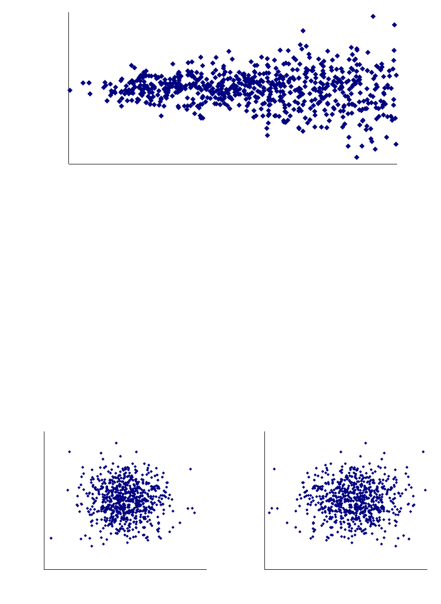
Regression for M&V: Reference Guide
33
Figure 5-2: Non-Constant Variance in Residuals
5.4.3. Uncorrelated with Independent Variables
The residuals should not show a strong correlation with any of the independent variables in the
regression model. To test the validity of this assumption, practitioners can use the same plots
examined in the previous section. The scatter plot of the residuals against the independent
variable(s) should show no linear patterns. The points should be randomly scattered around zero.
This relationship should also hold between the residuals and the predicted values of the dependent
variable. The left pane in Figure 5-3 shows residuals plotted against the independent variable, and
the right pane shows residuals plotted against the predicted values of the dependent variable. In
both cases, there are no trends – just random scatter around zero. (Note that practitioners may see
a linear trend when plotting residuals against actual values of the dependent variable, but this is
not worrisome.)
Figure 5-3: Residual Plots
-900
-600
-300
0
300
600
900
80 90 100 110 120 130 140 150 160 170 180 190 200
Residual
Independent Variable
-40
-30
-20
-10
0
10
20
30
40
60 80 100 120 140
Residual
Independent Variable
-40
-30
-20
-10
0
10
20
30
40
124 128 132 136 140 144
Residual
Predicted Values

Regression for M&V: Reference Guide
34
5.4.4. Independently Distributed (No Autocorrelation)
The residuals from a regression model are said to be independently distributed if the residual at
time is uncorrelated with the residual at time 1, 2, or any other period. If residuals are
found to be correlated with one another, they are said to suffer from autocorrelation or serial
correlation. Autocorrelation can be common in energy models, especially with data taken at short
intervals. For example, Figure 5-4 is a lag plot of residuals from a model using hourly data. It
charts the residuals (X axis) against the residuals from the prior hour (Y axis). Ideally, this plot
would reveal no trends. However, that is not the case – the strong relationship shown indicates that
this model suffers from autocorrelation. For this model, the autocorrelation should be accounted
for; if not, the uncertainty in the model will be underestimated.
Figure 5-4: Residual Lag Plot
The impact of autocorrelation is that the effective number of data points is fewer than the actual
number, since the information in each observation is not completely new. A consequence of this
is that the variability looks lower than it actually is, making some predictors look significant when
they are not. In the equations for the statistical tests, the effective number of data points needs to
be substituted for n, the actual number of data points.
Practitioners can estimate the effective number of data points (equation shown below) by first
calculating the first-order autocorrelation coefficient, (“rho”). This value is simply the
correlation between the residuals and the residuals for the prior time period. The effective number
of data points is then given by:
=
(
)
(
1
)
(
1 +
)
-4
-3
-2
-1
0
1
2
3
-4 -3 -2 -1 0 1 2 3
Residual Lag 1 hr (Watts per Square Foot)
Residual (Watts per Square Foot)

Regression for M&V: Reference Guide
35
Annex D of ASHRAE Guideline 14 suggests that autocorrelation can be ignored for values of
less than 0.5. Practitioners can also find a more dedicated discussion on autocorrelation (including
potential remedies) in the IPMVP Uncertainty Guide.
5.4.5. Other Plots
When analyzing residuals, there are a variety of other plots that practitioners may consider. A
residual time series plot, for example, plots the residuals against time. Such a plot may help identify
(1) regression outliers, (2) non-constant variance in the residuals, or (3) autocorrelation. Figure 5-5
shows a residual time series plot for a model that uses daily data. Residuals are plotted on the Y
axis and time (which is the date in this case) is plotted on the X axis. This figure is example of an
ideal residual time series plot – the spread is constant regardless of the time period, residuals tend
to hover around zero for the full time period (rather than hover above zero for a period of time,
then hovering below zero for the remainder of the time), and there are no alarming outliers. (Note
that a few spikes should be expected just by random chance.)
Figure 5-5: Residual Time Series Plot
5.5. Tables of Statistical Measures
Table 5-1 through Table 5-4, below, present the definitions of the relevant statistical measures,
their equation formulas, and their calculation in Microsoft Excel.
Table 5-1: Definitions of Regression Model Statistics
Regression Model Statistic Equation or Definition
n Number of points
p Number of parameters
df Degrees of freedom, = n - p
y
i
Actual y values
-50
-25
0
25
50
0 25 50 75 100 125 150 175 200 225 250 275 300 325 350
Residual
Time

Regression for M&V: Reference Guide
36
Regression Model Statistic Equation or Definition
Predicted y values
Y
avg
(or
) =
X
avg
(or
) =
SSQ
total
=
((
)
)
SSQ
reg
=
((
)
)
SSQ
res
(or SSE) =
((
)
)
SSQ
x
=
((
)
)
F
=
(
/
)
RMSE
=
/
CV(RMSE)
=
R-Squared
=
R-Squared = 1
(
)
Adjusted R-Squared
= 1
(
1
)
1
1
Net Determination Bias =
(
)
Confidence Half-Interval
= -
1
+
(
)
Prediction Half-Interval
= -
1 +
1
+
(
)
Table 5-2: Microsoft Excel Functions for Regression Model Statistics
Regression Model Statistic Microsoft Excel Function Excel LINEST (Where Applicable)
n = COUNT(XVals)
p 2
df = n-p
= INDEX(LINEST(Yvals,XVals,
TRUE,TRUE), 4,2)
Y
avg
= AVERAGE(Yvals)
X
avg
= AVERAGE(XVals)
SSQ
total
= DEVSQ(Yvals)
SSQ
reg
= DEVSQ(YvalsCalc)
= INDEX(LINEST(Yvals,XVals,
TRUE,TRUE), 5,1)

Regression for M&V: Reference Guide
37
SSQ
res
(or SSE) = SUM((Yvals-YvalsCalc)^2)
= INDEX(LINEST(Yvals,XVals,
TRUE,TRUE), 5,2)
SSQ
x
= DEVSQ(XVals)
F = DEVSQ(YvalsCalc)/(SUM((Yvals-
YvalsCalc)^2)/(n-p))
= INDEX(LINEST(Yvals,XVals,
TRUE,TRUE), 4,1)
RMSE
= SQRT(SUM((Yvals-
YvalsCalc)^2)/(n-p))
CV(RMSE) = SQRT(SUM((Yvals-YvalsCalc)
^2)/(n-p))/AVERAGE(Yvals)
R-Squared = RSQ(Yvals,XVals)
= INDEX(LINEST(Yvals,XVals,
TRUE,TRUE), 3,1)
R-Squared = RSQ(Yvals,XVals)
Adjusted R-Squared = 1-((1-RSQ(Yvals,XVals))*((n-1)/
(n-p-1)))
Net Determination Bias = SUM(Yvals-YvalsCalc)/SUM(Yvals)
Confidence Half-Interval
Evaluated at each x
Prediction Half-Interval
Evaluated at each x
Table 5-3: Definitions of Coefficient Statistics
Coefficient Statistic Equation or Definition
Confidence Level
Input required probability that the coefficient is not zero
t-Statistic, Critical From table
Intercept
=
Slope
=
(
)
(
)
((
)
)
Standard Error of Intercept
=
1
+
(
)
Standard Error of Slope
=
/()/
t-Statistic for Intercept = /( )
t-Statistic for Slope
= /( )
p-Value for Intercept —
p-Value for Slope
—
Table 5-4: Microsoft Excel Functions for Coefficient Statistics
Coefficient Statistic Microsoft Excel Function Excel LINEST (Where Applicable)
Confidence Level 0.95
t-Statistic, Critical
= T.INV.2T((1-ConfLvl)/2,n-p)
Intercept = INTERCEPT(Yvals,XVals)
Slope = SLOPE(Yvals,XVals)
= INDEX(LINEST(Yvals,XVals,
TRUE,TRUE), 1,2)

Regression for M&V: Reference Guide
38
Coefficient Statistic Microsoft Excel Function Excel LINEST (Where Applicable)
Standard Error of Intercept
= STEYX(Yvals,XVals)*SQRT
(1/n+Xavg^2/DEVSQ(XVals))
= INDEX(LINEST(Yvals,XVals,
TRUE,TRUE), 1,1)
Standard Error of Slope = STEYX(Yvals,XVals)*SQRT
(1/DEVSQ(XVals))
= INDEX(LINEST(Yvals,XVals,
TRUE,TRUE), 2,2)
t-Statistic for Intercept
= (INTERCEPT(Yvals,XVals))/
(STEYX(Yvals,XVals)*SQRT
(1/n+Xavg^2/DEVSQ(XVals)))
= INDEX(LINEST(Yvals,XVals,
TRUE,TRUE), 2,1)
t-Statistic for Slope
= (SLOPE(Yvals,XVals))/
(STEYX(Yvals,XVals)*SQRT
(1/DEVSQ(XVals)))
p-Value for Intercept = TDIST(ABS(INTERCEPT
(Yvals,XVals))/(STEYX(Yvals,
XVals)*SQRT(1/n+Xavg^2/
DEVSQ(XVals))),n-p,2)
p-Value for Slope = TDIST(ABS(SLOPE(Yvals,XVals))/
(STEYX(Yvals,XVals)*SQRT
(1/DEVSQ(XVals))),n-p,2)

Regression for M&V: Reference Guide
39
6. Example
6.1. Use of Monthly Billing Data in a 2-Parameter Model to
Evaluate Whether It Will Make a Satisfactory Baseline
Regression is commonly used to analyze monthly utility data. It is best applied to a package of
measures whose total savings is a relatively high percentage of the building’s baseline energy use.
It is important to remember that the energy use of buildings is typically dependent on weather.
More specifically, it can be dependent on the demand for cooling and heating. This is because
energy usage is usually higher when it is either very cold (heaters) or very hot (AC units), since
the temperature is far from the balance point.
In cases where only cooling or only heating is present or relevant, a simple 2-parameter (straight-
line) regression is often satisfactory.
Consider the case of schools in the Northwest, especially on the west side of the Cascade
Mountains. Many schools do not have cooling, and although cooling is not generally needed during
the school year, heating is. Therefore, a model of energy use versus average ambient temperature
or heating degree-days (HDD) may be appropriate.
Usually, degree-days are better than average-ambient-temperatures. An average temperature may
indicate little need for heating or cooling if it is near the balance point for the building. However,
a moderate average temperature can be made up of a series of cool temperatures and a series of
warm temperatures. During the times of cool temperatures, heating is needed. Therefore,
depending on climate, a better fit will typically be found by using degree-days. On the west side
of the Cascades in the Northwest, winter temperatures may be relatively constant over a day, and
almost always below a school building’s balance point, so the greatest difference between degree-
days and average temperature will be found in the spring and fall months.
The following analysis estimates the baseline for the electricity use of a group of modular
classrooms heated by heat pumps. The planned measure is a web-enabled programmable
thermostat. Prior similar projects have shown savings exceeding 45% of a building’s baseline
energy use.
The available data are the monthly electricity energy use (kWh) and ambient temperature during
the billing period. There are 24 months of data to be used for the baseline. The data to be used for
the regression will be normalized to average kWh per day in each billing period and average
heating degree-days per day in each billing period. The base temperature for heating degree-days
in this example is 65º F. (See Section 6.2 for a discussion of heating degree-days.)
The relevant equation is for a common 2-parameter ordinary least squares regression:
■
Y = β
1
+ β
2
X
1
where: Y = electricity use per day in the billing period

Regression for M&V: Reference Guide
40
β
1
= y-intercept – electricity use (kWh-per-day) for
a day with zero heating
degree-days
β
2
= slope – how much the energy use increases for a day as the temperature
decreases below 65º F (kWh-per-day per heating degree-day)
X
1
= average heating degree-days per day in the billing period
Table 6-1 provides the data for the project.
Table 6-1: Example Data for Classroom Heat Pump Project
End of Billing
Period
Billing Period
Duration in Days
Billed Usage
kWh
HDD in
Billing Period
09/24/2007
30 6,080 113
10/24/2007 30 7,330 311
11/21/2007 28 7,470 463
12/19/2007
28 10,000 669
01/23/2008 35 11,480 877
02/25/2008 33 11,420 782
03/26/2008
30 9,970 560
04/24/2008 29 7,840 561
05/20/2008
26 6,800 265
06/21/2008
32 5,980 268
07/23/2008 32 4,310 73
08/22/2008
30 3,330 57
The consumption and heating degree-days are standardized by the number of days in the billing
period (Table 6-2).
Table 6-2: Data Standardized by Days in the Billing Period
End of Billing
Period
Billing Period
Duration in
Days
Billed
Usage
kWh
HDD
in
Billing Period
Average kWh
per Day in
Billing Period
Average HDD
per Day in
Billing Period
09/24/2007
30 6,080 113 202.7 3.7
10/24/2007 30 7,330 311 244.3 10.4
11/21/2007
28 7,470 463 266.8 16.5
12/19/2007 28 10,000 669 357.1 23.9
01/23/2008 35 11,480 877 328.0 25.1
02/25/2008
33 11,420 782 346.1 23.7
03/26/2008 30 9,970 560 332.3 18.7
04/24/2008 29 7,840 561 270.3 19.4
05/20/2008
26 6,800 265 261.5 10.2
06/21/2008 32 5,980 268 186.9 8.4

Regression for M&V: Reference Guide
41
End of Billing
Period
Billing Period
Duration in
Days
Billed
Usage
kWh
HDD
in
Billing Period
Average kWh
per Day in
Billing Period
Average HDD
per Day in
Billing Period
07/23/2008 32 4,310 73 134.7 2.3
08/22/2008
30 3,330 57 111.0 1.9
Table 6-3 provides the Microsoft Excel formulas for the regression. Note that p in the term (n-p)
refers to the number of parameters, which is two for this simple linear regression.
Table 6-3: Microsoft Excel Formulas for the Regression
Output Formula
R-squared = RSQ(Yvals,XVals)
Number of Baseline Points, n = COUNT(YVals)
CV(RMSE)
= SQRT(SUM((Yvals-YvalsCalc)^2)/(n-p))/AVERAGE(Yvals)
Intercept at HDD=0
= INTERCEPT(Yvals,XVals)
Slope = SLOPE(Yvals,XVals)
Table 6-4 provides the Excel output:
Table 6-4: Microsoft Excel Output for Example Model
Output Data
R-squared
= 0.879
Number of Baseline Points, n = 12
CV(RMSE) = 11.7%
Intercept at HDD=0
= 132.24
Slope = 8.8678
Figure 6-1 shows the data graphed, with the regression equation and line included.

Regression for M&V: Reference Guide
42
Figure 6-1: Baseline Electricity Use vs. Heating Degree-Days
Next, the uncertainty needs to be calculated. The input confidence level used to calculate the
t-statistic will be 90%. The t-statistic will be used to get the confidence intervals, evaluated at each
value of X. To calculate the t-statistic, some intermediate calculations need to be made, as shown
in Table 6-5. In this table, p is the probability that the dependent variable is not significantly related
to the independent variable.
Table 6-5: Microsoft Excel Formulas for the Fit Statistics
Output Formula
Standard Error
= STEYX(Yvals,XVals)
Standard Error – Percent of Average
= STEYX(Yvals,XVals) / AvgY
Critical t-Statistic = TINV(1-ConfLvl,n-p)
Sum of Squares of Differences: X-avg(X)
= DEVSQ(XVals)
Standard Deviation of the Residuals = STDEV(Residuals)
t-Statistic = CONFIDENCE(1-ConfLvl,STDEV(Residuals),n)
p-Value
= TDIST(ABS(t_statistic),n-p,2)
Table 6-6 provides the Excel outputs for the goodness-of-fit statistics.
Table 6-6: Microsoft Excel Output for Example Fit Statistics
Output Data
Standard Error = 29.69
y = 8.8678x + 132.24
0
50
100
150
200
250
300
350
400
0 5 10 15 20 25 30
Average kWh per Day
During Billing Period
Average Heating Degree-Days During Billing Period
Baseline Data
Linear (Baseline Data)

Regression for M&V: Reference Guide
43
Standard Error – Percent of Average = 11.7%
Number of Baseline Points, n
= 12
Critical t-Statistic = 12
Sum of Squares of Differences: X-avg(X) = 1.81
Standard Deviation of the Residuals
= 818
t-Statistic = 28.3
p-Value = 13.44
Below is the equation for calculating the confidence intervals for the regression:
■
ΔY
confidence
= ±( t-statistic)*STEYX(Yvals,XVals)*SQRT(1/n+(X-
xAvg)^2/DEVSQ(XVals))
Table 6-7 provides the spreadsheet output, including the estimates for the confidence intervals of
the regression. Min Modeled is the modeled value minus the confidence half-interval. Max
Modeled is the modeled value plus the confidence half-interval.
Table 6-7: Example Model Estimates
Average HDD
per Day
in Billing
Period
Average kWh
per Day
in Billing
Period
Modeled
kWh
per Day
Residual 90%
Confidence
Half-Interval
Minimum
Modeled
kWh
per Day
Maximum
Modeled
kWh
per Day
3.7
202.7 165.5 37.2 24.3 141.2 189.8
10.4 244.3 224.2 20.1 16.7 207.5 241.0
16.5 266.8 278.8 -12.0 16.4 262.4 295.3
23.9
357.1 344.1 13.1 24.7 319.4 368.8
25.1 328.0 354.4 -26.4 26.5 327.9 380.8
23.7
346.1 342.5 3.6 24.5 318.0 366.9
18.7
332.3 297.7 34.6 18.2 279.6 315.9
19.4 270.3 303.9 -33.6 18.9 285.1 322.8
10.2
261.5 222.4 39.1 16.9 205.6 239.3
8.4 186.9 206.6 -19.7 18.4 188.2 225.1
2.3 134.7 152.6 -17.9 26.5 126.1 179.0
1.9
111.0 149.0 -38.0 27.1 121.9 176.1
Total 3,041.8 3,041.8 0.0 258.9 2,782.8 3,300.7
Figure 6-2 provides the scatter chart again, including the lines of 90% confidence intervals.

Regression for M&V: Reference Guide
44
Figure 6-2: Baseline Electricity Use vs. Heating Degree-Days with Confidence Intervals
Note that the regression appears to reproduce the baseline totals. However, these values are for the
average kWh-per-day, not for the total energy use over the year. Yet each point does not represent
the same number of days; consequently, the best approach would have been to use a weighted
regression. Because a weighted regression was not used, the model’s bias should be checked.
To complete the model and check the bias, the modeled values for kWh-per-day are multiplied by
the number of days in the billing period. The actual kWh values are reproduced in Table 6-8 for
comparison with the modeled values.
Table 6-8: Example Model Estimates with Actual Observations
Average
HDD per
Day
in Billing
Period
Av
erage
kWh
per Day
in Billing
Period
Modeled
kWh
per Day
Residual 90%
Confidence
Half-
Interval
Minimum
Modeled
kWh
per Day
Maximum
Modeled
kWh
per Day
Actual
kWh
Modeled
kWh
3.7
202.7 165.5 37.2 24.3 141.2 189.8 6,080 4,964
10.4
244.3 224.2 20.1 16.7 207.5 241.0 7,330 6,727
16.5 266.8 278.8 -12.0 16.4 262.4 295.3 7,470 7,807
23.9
357.1 344.1 13.1 24.7 319.4 368.8 10,000 9,634
25.1 328.0 354.4 -26.4 26.5 327.9 380.8 11,480 12,403
23.7 346.1 342.5 3.6 24.5 318.0 366.9 11,420 11,301
18.7
332.3 297.7 34.6 18.2 279.6 315.9 9,970 8,932
19.4 270.3 303.9 -33.6 18.9 285.1 322.8 7,840 8,814
10.2 261.5 222.4 39.1 16.9 205.6 239.3 6,800 5,783
y = 8.8678x + 132.24
0
50
100
150
200
250
300
350
400
0 5 10 15 20 25 30
Average kWh per Day
During Billing Period
Average Heating Degree-Days During Billing Period
Baseline Data
Lower Confidence Line
Upper Confidence Line

Regression for M&V: Reference Guide
45
8.4 186.9 206.6 -19.7 18.4 188.2 225.1 5,980 6,612
2.3
134.7 152.6 -17.9 26.5 126.1 179.0 4,310 4,883
1.9 111.0 149.0 -38.0 27.1 121.9 176.1 3,330 4,469
Total 3,041.8 3,041.8 0.0 258.9 2,782.8 3,300.7 92,010 92,331
So, what is the bias in the model?
■
Net Determination Bias Error (NDBE): NDBE
NDBE = (92,331 – 92,010) / 92,331
NDBE = 0.3%
The model predicts 0.3% higher energy use than the actual data.
ASHRAE Guideline 14 does not accept a model with bias >0.005%, so this model would be
rejected. However, the uncertainty in the model is much, much greater than the bias, and the
savings are expected to be much, much greater than the uncertainty. Thus, this model is acceptable:
■
Modeled Uncertainty = ± (92,331 – 84,436) / 92,331 = ± 8.6%.
The expected energy savings for this measure is at least 45%. Since the uncertainty is low relative
to the expected savings, this baseline model would be acceptable for projecting energy use under
post-implementation conditions and could be used in the calculation of energy savings.
6.2. Background on Heating and Cooling Degree-Days
(HDD and CDD)
Heating degree-days are a measure of how much cold weather there is in a specific period. The
average daily temperature is determined for each day. The average temperature is then compared
to a base temperature (often 65º F). If the average temperature (when only daily data are available,
typically the average of the daily high and the daily low) is 55º F for a day, and the base is 65º F,
then that day contributes 10 HDD to the period. The HDD for each day in the period (typically a
calendar month or a utility billing period) are summed to create a single data point for the month.
If the temperature difference for a day is negative, it is recorded as 0.
■
HDD
n
=
Note that while HDD and CDD are often reported with a base or balance point of 65º F, results
can often be improved by experimenting with different base temperatures. The base temperature
should generally be the average temperature at which the building does not require any heating or
∑
∑
−
∗=
i
i
i
ii
E
EE )
ˆ
(
100
( )
+
∑
−
n
i
ibase
TT
Regression for M&V: Reference Guide
46
cooling – the balance point temperature. For most commercial buildings, this temperature will
typically be between 55° and 60º F, depending on building size, operating schedule, and other
parameters. If regression models are created separately for occupied and unoccupied periods, the
balance point temperature will be different for each: for the occupied period, it may be near 55º F,
and for the unoccupied period it may be near 65º F.

Regression for M&V: Reference Guide
47
7. Minimum Reporting Requirements
This document is a reference guide, a companion to the M&V protocols. Below are the minimum
reporting requirements for the use of regressions within protocols. The overall M&V approach
should be described according to the minimum reporting requirements of the protocol used. Please
see the protocols for minimum reporting requirements.
These are the essential reporting requirements for regressions within an M&V plan and verification
report:
Data: variables, interval of observation – such as monthly, number of observations, or
length of measurement period
Model: the proposed or final model and alternative models proposed or tested (the
verification report should include estimated model parameters)
Model Statistics: statistics for assessing goodness of fit (proposed and, in the verification
report, calculated statistics for final model)
Discussion: why the final model was selected or weaknesses of the alternative models
tested

Regression for M&V: Reference Guide
48
8. References and Resources
ASHRAE. 2004. ASHRAE RP-1050 – Inverse Modeling Toolkit.
See: Kissock, J., J. Haberl, and D. Claridge. Inverse Modeling Toolkit: Numerical
Algorithms.
Purchase at: https://store.accuristech.com/standards/kc-03-02-2-rp-1050-inverse-model-
toolkit-application-and-testing?product_id=1717581
ASHRAE. 2023. ASHRAE Guideline 14-2023 – Measurement of Energy, Demand, and Water
Savings. Atlanta, Ga.: American Society of Heating, Refrigerating and Air-Conditioning
Engineers.
Purchase at: https://store.accuristech.com/standards/ashrae-guideline-14-2023-
measurement-of-energy-demand-and-water-savings?product_id=2569793
ASHRAE. 2014. ASHRAE RP-1404 – Measurement, Modeling, Analysis and Reporting
Protocols for Short-term M&V of Whole Building Energy Performance. Atlanta, Ga.:
American Society of Heating, Refrigerating and Air-Conditioning Engineers.
Purchase at: https://store.accuristech.com/standards/rp-1404-measurement-modeling-
analysis-and-reporting-protocols-for-short-term-m-v-of-whole-building-energy-
performance?product_id=1872406
Brase, Charles Henry, and Corrinne Pellillo Brase. 2009. Understandable Statistics: Concepts
and Methods (9th Ed.). New York, N.Y.: Houghton Mifflin.
California Commissioning Collaborative. 2008. Guidelines for Verifying Existing Building
Commissioning Project Savings, Using Interval Data Energy Models: IPMVP Options B
and C. 2008. California Commissioning Collaborative.
Available at: https://facilityenergysolutions.com/publications
IPMVP. 2022. International Performance Measurement and Verification Protocol Core
Concepts, March 2022. EVO 10000 – 1:2022. Washington, D.C.: Efficiency Valuation
Organization.
Available at: https://evo-world.org/en/products-services-mainmenu-en/protocols/ipmvp
IPMVP. 2012. International Performance Measurement and Verification Protocol Volume I:
Concepts and Options for Determining Energy and Water Savings. EVO 10000 – 1:2012.
Washington, D.C.: Efficiency Valuation Organization.
Available at: https://evo-world.org/en/products-services-mainmenu-en/protocols/ipmvp
IPMVP. 2016. Core Concepts International Performance Measurement and Verification
Protocol. EVO 10000 – 1:2016. Washington, D.C.: Efficiency Valuation Organization.
Available at: https://evo-world.org/en/products-services-mainmenu-en/protocols/ipmvp
IPMVP. 2018. Uncertainty Assessment, International Performance Measurement and
Verification Protocol. EVO 10100-1:2018. Washington, D.C.: Efficiency Valuation
Organization.
Regression for M&V: Reference Guide
49
Available at: https://evo-world.org/en/products-services-mainmenu-en/protocols/ipmvp
Haberl, J., A. Sreshthaputra, D. Claridge, and J. Kissock. 2003. Inverse Model Toolkit:
Application and Testing. KC-03-02-2 (RP-1050). Atlanta, Ga.: American Society of
Heating, Refrigerating and Air-Conditioning Engineers.
Purchase at: https://store.accuristech.com/ashrae/standards/kc-03-02-2-rp-1050-inverse-
model-toolkit-application-and-testing?product_id=1717581
Hardy, Melissa A. 1993. Regression with Dummy Variables. Newbury Park, Calif.: Sage.
Kissock, J., J. Haberl, and D. Claridge. 2004. RP-1050 – Development of a Toolkit for
Calculating Linear, Change-Point Linear and Multiple-Linear Inverse Building Energy
Analysis Models. Atlanta, Ga.: American Society of Heating, Refrigerating and Air-
Conditioning Engineers.
Available at: https://oaktrust.library.tamu.edu/handle/1969.1/2847
Kissock, J., J. Haberl, and D. Claridge. 2004. Inverse Modeling Toolkit: Numerical Algorithms.
KC-03-02-1 (RP-1050). Atlanta, Ga.: American Society of Heating, Refrigerating and
Air-Conditioning Engineers.
Purchase at: https://store.accuristech.com/ashrae/standards/kc-03-02-1-rp-1050-inverse-
modeling-toolkit-numerical-algorithms?product_id=1717580
NIST/SEMATECH. 2011. Engineering Statistics Handbook (NIST/SEMATECH e-Handbook of
Statistical Methods). Gaithersburg, Md.: National Institute of Standards and Technology.
Available at: http://www.itl.nist.gov/div898/handbook/index.htm.
Stevens, James. 2002. Applied Multivariate Statistics for the Social Sciences. Mahwah, N.J.:
Lawrence Erlbaum Associates.
TecMarket Works Team. California Energy Efficiency Evaluation Protocols: Technical,
Methodological, and Reporting Requirements for Evaluation Professionals. April 2006.
San Francisco, Calif.: California Public Utilities Commission.
Available at:
https://www.calmac.org/publications/EvaluatorsProtocols_Final_AdoptedviaRuling_06-
19-2006ES.pdf
Thompson, Steven K. 2002. Sampling. (2nd Ed.). New York, N.Y.: John Wiley & Sons, Inc.

Regression for M&V: Reference Guide
50
9. Appendix: Glossary of Statistical Terms
This Glossary provides definitions for the statistical terms used in this Regression Reference
Guide. Additional M&V terms are defined in the companion document Glossary for M&V:
Reference Guide.
Accuracy: An indication of how close the measured value is to the true value of the quantity in
question. Accuracy is not the same as precision.
Adjusted R
-square (
2
R
): A modification of R
2
that adjusts for the number of independent
variables
(explanatory terms) in a model. The adjusted R
2
only increases if the additional
independent variables improve the model more than by random chance. It is calculated by taking
R
2
and dividing it by the associated degrees of freedom. Or as described below:
= 1
Autocorrelation Coefficient
: See Autocollinearity
A
utocollinearity: The serial correlation over time of predictor values in a time series model.
To
calculate autocollinearity, R
-
squared is first calculated for the correlation between the residuals
and the residuals for the prior period. The autocorrelation coefficient
ρ
is then the square root of
this value.
19
Autocollinearity is calculated as:
22
( )( )
( )( )
ii
i
ii
ii
x xy y
xx yy
ρ
−−
=
−−
∑
∑∑
Categorical Variables:
Variables that have discrete values and are not continuous.
Categorical
variables include things like daytype (weekday or weekend, or day of week), occupancy (occupied
or unoccupied), and equipment status (on or off).
For example, occupancy (occupied or
unoccupied) is a categorical variable, while number of occupants is a continuous variable.
Coefficient of Variation (CV)
:
An indication of how much variability or randomness there is with
any given data set. It quantifies variation within the population relative to the average and is
dimensionless. The larger it is, the more variation there is in the population relative to the average.
It is calculated as the ratio of the standard deviation to the average
:
=
19
Note, the English spelling of the Greek letter ρ is rho, not to be confused with “p.”

Regression for M&V: Reference Guide
51
Coefficient of Variation
of the Root-Mean Squared Error [CV(RMSE)]:
A measure that
describes how much variation or randomness there is between the data and the model, calculated
by dividing the root
-mean squared error (RMSE) by the average y-value. It is calculated as:
(
)
=
1
(
)
(
)
/
Confidence Interval:
A range of uncertainty expected to contain the true value within a specifi
ed
probability. The probability is referred to as the confidence level.
Confidence Level: A population parameter used to indicate the reliability of a statistical estimate.
The confidence interval expresses the assurance (probability) that given correct model selection,
the true value of interest resides within the proportion expressed by the confidence interval.
Continuous Variables: Variables that are numeric and can have any value within the range of
encountered data (that is, measurable things such as energy usage or ambient temperature).
Degree Day
: A degree-day is a measure of the heating or cooling load on a facility
created by
outdoor temperature. When the mean daily outdoor temperature is one degree below a stated
reference temperature such as 18°C, for one day, it is defined that there is one heating degree
-
day.
If this temperature difference prevailed for ten days
, there would be ten heating degree-
days
(HDD)
counted for the total period. If the temperature difference were to be 12 degrees for ten
days, 120 heating degree
-days would b
e counted. When the ambient temperature is below the
reference temperature
, it is defined that heating degree-
days are counted. When ambient
temperatures are above the reference, cooling degree
-days (CDDs)
are counted. Any reference
temperature may be used for recording degree
-
days, though it is usually chosen to reflect the
temperature at which a particular building no longer needs heating or cooling.
Dependent Variable:
The variable that changes in relationship to alterations of the independent
variable. In energy efficiency, energy usage is typically treated as the dependent variable,
responsive to the manipulation of conditions (independent variables).
Homoscedasticity:
(Also known as Homogeneity of Variance.)
Within linear regression, this
means that the variance of the dependent values around the regression line is constant for all values
of the independent variable.
Independent
Variable: Also termed an explanatory or exogenous variable; a
factor that is
expected to have a measurable impact on the
dependent, or outcome variable (such
energy use of
a system or facility).
Mean
: The most widely used measure of the central tendency of a series of observations.
The
Mean
() is determined by summing the individual observations (
)
and dividing by the total
number of observations (
), as follows:

Regression for M&V: Reference Guide
52
Mean Bias Error (MBE)
: The Mean Bias Error
is an indication of overall bias in a regression
model. Positive
MBE indicates that regression estimates tend to overstate the actu
al values. It is
calculated as:
=
(
)
Mean Model:
(Also known as a Single Parameter Model
.) A model that estimates the mean of
the dependent variable.
Multicollinearity: A statistical occurrence where two or more predictor variables in a multiple
regression model are highly correlated (there are exact linear relationships between two or more
explanatory variables). Allowing multicollinearity in a model can lead to incorrect inferences from
the model.
Net Bias:
Where there exists net bias, modeled or predicted energy usage will differ from actual
energy usage for the period examined.
Net Determination Bias
Error (NDBE): T
he percentage error in the energy use predicted by the
model compared to the actual energy use.
See Normalized Mean Bias Error.
= 100
Normal Distribution:
A continuous and symmetric population distribution in
which the
frequency of occurrence decreases exponentially as values deviate from the mean (or central)
value.
In a regression equation, the distribution of errors (residuals) at a given value of x
is a normal
distribution and the mean of residuals is zero. It is also referred to as a Gaussian or bell curve.
Normalized Mean Bias Error (
NMBE): Similar to Net Determination Bias
but adjusted for the
number of parameters in the model
. The Normalized Mean Bias Error
is an indication of overall
bias in a regression model. Positive
MBE
indicates that regression estimates tend to overstate the
actual values. It is calculated as:
= 100
(
)
Ordinary Least Squares (OLS):
A mathematical
procedure to solve for the set of coefficients
that minimize the sum of the squared differences between the raw data and the fitted linear trend.
OLS
is the most common form of regression modeling and the default approach in most software
packages.
Outliers:
Data points that do not conform to the typical distribution. Graphically, a
n outlier
appears to deviate markedly from other members of the same sample.
Over
specified Model:
A model with added independent variables that are not statistically
significant or are possibly correlated with other independent variables.

Regression for M&V: Reference Guide
53
p
-value: T
he probability that a coefficient or dependent variable is not related to the independent
variable. Small
p-
values, then, indicate that the independent variable or coefficient is a significant
(important) predictor of the dependent variable in a regression model. The
p-
value is an alternate
way of evaluating the
t-statistic for the significance of a regression coefficient and
is expressed as
a probability.
Precision: The indication of the closeness of agreement among repeated measurements; a measure
of the repeatability of a process. Any precision statement about a measured value must include a
confidence level. A precision of 10% at 90% confidence means that we are 90% certain the
measured values are drawn from samples that represent the population and that the “true” value is
within ±10% of the measured value. Because precision does not account for bias or instrumentation
error, it is an indicator of predicted accuracy only given the proper design of a study or experiment.
R
-Squared (R
2
): (Also known as the Coefficient of Determination.) R
2
is the measure of how well
future outcomes are likely to be predicted by the model. It illustrates how well the independent
variables explain variation in the dependent variable.
R
2
values range from 0 (indicating none of
the variation in the dependent variable is associated with variation in any of the independent
variables) to 1 (indicating
all
the variation in the dependent variable is associated with variation in
the independent variables, a “perfect fit” of the regression line to the data)
. It is calculated as:
= 1
Regression Analysis: A mathematical technique that extracts parameters from a set of data to
describe the correlation relationship of measured independent variables and dependent variables.
Regression Model: A mathematical model based on statistical analysis where the dependent
variable is regressed on the independent variables which are said to determine its value. In so
doing, the relationship between the variables is estimated from the data used. A simple
linear
regression is calculated as:
=
+
+
, where i = 1,…, n
Reliability:
When used in energy evaluation, refers to the likelihood that the observations can be
replicated.
Residual:
The difference between the predicted and actual value of the dependent variable. In
other words, whether a point is above or below the regression line is a matter of chance and is not
influenced by whether another point is above or below the line. Estimated by subtracting the data
from the sample
mean:
ˆ
i
XX
ε
= −

Regression for M&V: Reference Guide
54
Root Mean Squared Error
(RMSE): A
n indicator of the scatter, or random variability, in the
data, and hence is an average of how much an actual
y-value differs from the predicted y-value
. It
is the standard deviation of errors of prediction about the regression line. The RMSE is calculated
as:
=
(
) =
(
)
Standard Deviation (s): The square root of the variance, which brings the variability measure
back to the units of the data.
(With variance units in kWh
2
, the standard deviation units are kWh.)
The sample standard deviation (
s) is calculated as:
Standard Error (SE):
A
n estimate of the standard deviation of the coefficient. For simple linear
regression, it is calculated separately for the slope and intercept: there is a standard error of the
intercept
and standard error of the slope. SE is calculated as:
=
Standard Error of the Coefficient
: Similar to the RMSE
but calculated for a single coefficient
rather than the complete model
.
This measures the degree to which the coefficient estimate may
change if the full process was to be repeated.
t
-statistic:
A measure of the probability that the value (or difference between two values) is
statistically valid. The calculated
t-statistic can be compared to critical t-values from a t-table
. The
t
-statistic is inversely related to the p-value; a high t-statistic
(t>2) indicates a low probability that
random chance has introduced an erroneous result
. Within regression, the t-
statistic is a measure
of the significance for each coefficient (and, therefore, of each independent variable) in the model.
The l
arger the t-statistic, the more significant the coefficient is to the estimation of
the dependent
variable
. The t-statistic is calculated as:
=
. . (
)
Uncertainty:
The range or interval of doubt surrounding a measured or calculated value within
which the true value is expected to fall within some stated degree of confidence. Uncertainty in
regression analysis can come from multiple sources,
including measurement uncertainty
and
regression uncertainty.

Regression for M&V: Reference Guide
55
Variance (S
2
): A
measure of the average distance between each of a set of data points and their
mean value, and it is equal to the sum of the squares of the deviation from the mean value, or the
square of the standard deviation
. Variance is computed as follows:
=
(
)
1
Weighted Regression:
A form of regression used when individual data points are weighted
to
represent more data than other points. An example is billing
-
period analysis, where billing periods
may have different numbers of days and billing periods with more days are adjusted upward in
weight relative to
periods with fewer days. (
Also, a form of regression used when data do not have
equal weight in a model because error is not expected to be constant across all observations.)
