1
An Updated User’s Guide to SOFR
The Alternative Reference Rates Committee
February 2021
2
Executive Summary
This note is intended to help explain how market participants can use SOFR in cash products. The
ARRC has stated that those who are able to use SOFR should not wait for forward-looking term rates
in order to transition, and the note lays out a number of considerations that market participants
interested in using SOFR will need to consider:
• Financial products either explicitly or implicitly use some kind of average of SOFR, not a single
day’s reading of the rate, in determining the floating-rate payments that are to be paid or
received. An average of SOFR will accurately reflect movements in interest rates over a given
period of time and smooth out any idiosyncratic, day-to-day fluctuations in market rates.
• Issuers and lenders will face a technical choice between using a simple or a compound average of
SOFR as they seek to use SOFR in cash products. In the short-term, using simple interest
conventions may be easier since many systems are already set up to accommodate it. However,
compounded interest would more accurately reflect the time value of money, which becomes
a more important consideration as interest rates rise, and it can allow for more accurate
hedging and better market functioning.
• Users need to determine the period of time over which the daily SOFRs are observed and
averaged. An in advance structure would reference an average of SOFR observed before the
current interest period begins, while an in arrears structure would reference an average of
SOFR over the current interest period.
• SOFR in advance is operationally easier to implement, but SOFR in arrears will reflect
movements in rates contemporaneously. An average of SOFR in arrears will reflect what
actually happens to interest rates over the period; however it provides very little notice before
payment is due. There have been a number of conventions designed to allow for a longer
notice of payment within the in arrears framework. These include payment delays, lookbacks,
and lockouts, and, as described in the note, different markets have successfully adopted each
of these. The note also discusses conventions for in advance payment structures and hybrid
models that can substantially reduce the basis relative to in arrears while still providing
borrowers the same length of notice that they have with LIBOR.
The note also explains the interaction between SOFR and the type of forward-looking term rates
that the ARRC has set a goal of seeing produced once SOFR derivative markets develop sufficient
depth. While these term rates can be a useful tool for some and an integral part of the new
ecosystem, hedging these rates will also tend to entail more costs than using SOFR directly and their
use must be consistent with the functioning of the overall financial system. For this reason, the
ARRC sees some specific productive uses for a forward-looking SOFR term rate, in particular as a
fallback for legacy cash products referencing LIBOR and in loans where the borrowers otherwise
have difficulty adapting to the new environment.

3
Background
In 2014, the Federal Reserve convened the Alternative Reference Rates Committee (ARRC) and
tasked the group with identifying an alternative to U.S. dollar LIBOR that was a robust, IOSCO-
compliant, transaction-based rate derived from a deep and liquid market. In 2017, the ARRC fulfilled
this mandate by selecting the Secured Overnight Financing Rate, or SOFR. SOFR is based on
overnight transactions in the U.S. dollar Treasury repo market, the largest rates market at a given
maturity in the world. National working groups in other jurisdictions have similarly identified
overnight nearly risk-free rates (RFRs) like SOFR as their preferred alternatives.
SOFR has a number of characteristics that LIBOR and other similar rates based on wholesale term
unsecured funding markets do not:
• It is a rate produced by the Federal Reserve Bank of New York for the public good;
• It is derived from an active and well-defined market with sufficient depth to make it
extraordinarily difficult to ever manipulate or influence;
• It is produced in a transparent, direct manner and is based on observable transactions, rather
than being dependent on estimates, like LIBOR, or derived through models; and
• It is derived from a market that was able to weather the global financial crisis and that the
ARRC credibly believes will remain active enough in order that it can reliably be produced in
a wide range of market conditions.
However, SOFR is also new, and many are unfamiliar with how to use it. SOFR is also an overnight
rate, and while the ARRC believes that most market participants can adapt to this by using compound
or simple averaging over the relevant term, the ARRC has at the same time set a goal of seeing an
administrator produce a forward-looking term rate based on SOFR derivatives (once these markets
develop to sufficient depth) in order to aid those cash market participants who may have greater
difficulty in adapting to an overnight rate.
The national working groups in the other currency jurisdictions each independently reached the same
conclusion that there were no viable robust term rate alternatives to LIBOR. Like the ARRC, each
has chosen either an unsecured or secured overnight rate, depending on the characteristics of their
national markets (see Table 1).
1
Table 1: Selected RFRs
U.S. Dollar
SOFR
Overnight secured repo rate
Sterling
SONIA
Overnight unsecured rate
Japanese Yen
TONA
Overnight unsecured rate
Euro
ESTER
Overnight unsecured rate
Swiss Franc
SARON
Overnight secured repo rate
1
Further information on the work of each of the national working groups in other currency jurisdictions can be found in
the FSB’s Progress Report on Reforming Major Interest Rate Benchmarks
, October 2017.

4
This note is intended to help explain how market participants can use SOFR in cash products and to
explain the forward-looking term rates the ARRC seeks to see published in the future and where the
ARRC believes those rates can be most productively used. The term rates can be a useful tool for
some and an integral part of the new ecosystem; but their use also needs to be consistent with the
functioning of the overall financial system. In particular, those who are able to use SOFR should not
wait for the term rates in order to transition.
2
The LIBOR transition will be challenging, and it is not
in the interest of market participants to put off taking action nor can the ARRC guarantee that an
administrator can produce a robust, IOSCO-compliant forward-looking term rate before LIBOR
stops publication. The ARRC sees some specific uses, in particular as a fallback for legacy cash
products referencing LIBOR and in loans where the borrowers otherwise have difficulty in adapting
to the new environment, where the term rates can be most productively used. For many other
purposes, the ARRC believes it should be possible to use compound or simple averages of SOFR and
that many users will come to find it more convenient to do so once they become more familiar with
the new environment.
A.
SOFR
SOFR is published on a daily basis by the Federal Reserve Bank of New York (FRBNY), in
cooperation with the Office of Financial Research, and reflects the cost of overnight borrowing and
lending in the U.S. Treasury repo market. Borrowing in this market reflects the best measure of the
private sector risk-free rate, because it is collateralized with U.S. Treasury securities, which the lender
returns once the borrower returns the cash borrowed. SOFR is a fully transactions-based rate and has
the widest coverage of any Treasury repo rate available, incorporating tri-party repo data, the Fixed
Income Clearing Corporation’s (FICC) GCF Repo data, and bilateral Treasury repo transactions
cleared through FICC.
3
Throughout 2020, the average daily volume of transactions underlying SOFR
was close to $1 trillion, representing the largest rates market at any given tenor in the United States.
Because of its range of coverage, SOFR is a good representation of general funding conditions in the
overnight Treasury repo market. As such, it reflects an economic cost of lending and borrowing
relevant to the wide array of market participants active in these markets, including not only broker-
dealers, but also money market funds, asset managers, insurance companies, securities lenders, and
pension funds. SOFR moves closely with other available repo rates and has tended to lie in the middle
of the range between other available repo rates. SOFR is generally a few basis points higher than rates
based only on tri-party transactions (such as the Bank of New York Mellon’s Treasury Tri-Party Repo
Index or the tri-party general collateral rate produced by FRBNY) but is generally lower and less
volatile than DTCC’s Treasury GCF Repo Index.
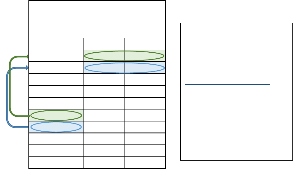
SOFR is calculated as a volume-weighted median of transaction-level data observed over the course
of a business day and is published on the FRBNY website at approximately 8:00 a.m. ET on the next
business day (see the accompanying figure). Looked at another way, SOFR is published on the day
that the overnight repo transaction is to be repaid rather than on the day that the transaction is entered
into. This publication schedule is due to the need to receive and fully vet the large amounts of data
2
The FSB has recognized that there may be a role for these types of forward-looking term rates, but the FSB has also
stated that it considers that the greater robustness of overnight rates like SOFR makes them a more suitable alternative
than these forward-looking term rates in the bulk of cases.
3
Further details on the structure of the U.S. Treasury repo market is available in the ARRC’s Second Report; see also
Bowman, Louria, McCormick and Styczynski (2017).

5
underlying SOFR before the rate is published. SOFR is published for the business days that the
Treasury repo market is open on, which are generally U.S. government securities secondary-market
trading days as determined by SIFMA
4
Although SOFR is published at about 8:00 a.m. ET, if any errors are subsequently discovered in the
transaction data in the calculation process that underlies it, or if any missing data subsequently became
available, then SOFR may be republished on the same day. In such cases, the affected rate may be
republished at approximately 2:30 p.m. ET. Rate revisions will only be effected on the same day as
initial publication and will only be republished if the change in the rate exceeds one basis point. To
date, there have been no rate republications for SOFR, but if at any time a rate is revised, a footnote
would indicate the revision.
5
4
SIFMA’s calendar of government securities trading days can be found at
https://www.sifma.org/resources/general/holiday-schedule/#US
.
5
Although SOFR has not been republished, on May 31, 2019, it was published based on FRBNY’s contingency rate
calculation methodology. This methodology involves the use of a highly detailed survey of Primary Dealer’s repo
borrowing activity conducted by FRBNY every day. More information and this event and a summary of FRBNY’s data
contingency procedures can be found on FRBNY’s website.
4/16/2019
SOFR is published on every U.S.
business day at approximately
8:00am EST. Because the Fed has
the ability to correct and republish
this rate until 2:30pm New York
City Time each day, users may wish
to reference the rate after this
time (e.g. 3:00pm)
The SOFR rate published on any
day represents the rate on repo
transactions entered into on the
previous business day and the date
associated with each rate reflects
the date of the underlying
transactions rather than the date
of publication.

6
In addition to producing SOFR, the Federal Reserve Bank of New York also publishes 30-day, 90-
day, and 180-day averages of SOFR and a SOFR Index daily on its website.
SOFR averages can be used either in advance or in arrears (concepts discussed further below) depending
on whether the averages are applied at the start or end of an interest period, but they are more likely
to be used in advance. They are calculated based on ISDA’s compound SOFR formula (described in
the Appendix), although the calculations for the averages may start on a weekend or holiday in order
to ensure that they cover a fixed number of days, and in that respect they differ from the standard
convention in the SOFR OIS market which would always start and stop on a business day. To allow
users to calculate a compound SOFR based on ISDA’s definitions over any start and ending date, for
example a monthly compound average based on the modified following business day convention,
FRBNY also publishes the SOFR Index. The Index, and how it can be interpolated to calculate a
compound average over a period that starts or stops on a nonbusiness day, is covered further in the
Appendix.
SOFR and the SOFR averages and Index are available both on FRBNYs website and also through an
API or through various data providers. Documentation for these rates can be found on the FRBNY
website, including policies and procedures and detailed evidence of IOSCO compliance. In addition
to SOFR, FRBNY produces a number of daily statistics, including the volume of transactions
underlying SOFR and selected percentiles of the rates observed across transactions, to aid market
participants in judging the quality of the rate.
B.
How Can Financial Products Use Overnight Rates?
Although many market participants have become accustomed to using term IBORs, they are a
relatively new phenomenon, and financial markets were able to function perfectly well before these
rates were widely adopted. There is in fact a long history of use of overnight rates in financial
instruments. In the United States, futures referencing the effective federal funds rate (EFFR) have
traded for more than 30 years and overnight index swaps (OIS) referencing EFFR have traded for
almost 20 years. Banks in the United States also have a history of offering loans based on the Prime
Rate, which is essentially an overnight rate, or overnight LIBOR, and there have been floating rate
Historical SOFR Data
FRBNY, in cooperation with the Office of Financial Research, began publishing
SOFR on April 3, 2018, but there is a longer history of repo rate data based on
several sources that have been made available by FRBNY. Prior to the start of
official publication, FRBNY also released data from August 2014 to March 2018
representing modeled, pre-production estimates of SOFR that are based on the
same basic underlying transaction data and methodology that now underlie the
official publication. While the full set of data sources required to calculate SOFR
did not exist prior to August 2014, FRBNY has also separately released a much
longer historical data series based on primary dealers' overnight Treasury repo
borrowing activity. Bowman (2017) provides evidence that this historical data
should be a good proxy for how a rate like SOFR would have behaved over a
longer period of time.

7
notes (“FRN”) issued based on the EFFR or, more recently, SOFR. Other countries have similar
experiences; for example, in Canada, most floating-rate mortgages are based on overnight rates.
Averaged Overnight Rates
Many financial products have used overnight rates as benchmarks, but one key thing to keep in mind
is that these financial products either explicitly or implicitly use some kind of average of the overnight
rate, not a single day’s reading of the rate, in determining the floating-rate payments that are to be paid
or received.
There are two essential reasons why financial products use an average of the overnight rate:
• First, an average of daily overnight rates will accurately reflect movements in interest rates
over a given period of time. For example, SOFR futures and swaps contracts are constructed
to allow users to hedge future interest rate movements over a fixed period of time, and an
average of the daily overnight rates that occur over the period accomplishes this.
• Second, an average overnight rate smooths out idiosyncratic, day-to-day fluctuations in market
rates, making it more appropriate for use.
This second point can be seen in Figure 1. On a daily basis, SOFR can exhibit some amount of
idiosyncratic volatility, reflecting market conditions on any given day, and a number of news articles
pointed to the jump in SOFR and other overnight repo rates in the fall of 2019. However, although
people often focus on the type of day-to-day movements in overnight rates shown by the black line
in the figure, it is important to keep in mind that the type of averages of SOFR that are referenced in
financial contracts are much smoother than the movements in overnight SOFR.
0
1
2
3
4
5
6
2015 2016 2017 2018 2019 2020
Figure 1: Movements in SOFR versus SOFR Averages
SOFR
30-Day SOFR
90-Day SOFR
180-Day SOFR
Percent
Source: Federal Reserve Bank of New York; Federal Reserve Board staff calculations. Data from August 2014 to
March 2018 represent modeled, pre-production estimates of SOFR.

8
The amount of daily volatility in SOFR can change over time and depends on a number of factors,
including the monetary policy framework and day-to-day fluctuations in supply and demand, but
regardless of these factors, using an averaged overnight rate smooths out almost all of this type of
volatility. As was emphasized in the ARRC’s Second Report and is still the case today even over the
year end, a three-month average of SOFR is less volatile than 3-month LIBOR (Figure 2). This was
true even in 2019 over the period when overnight repo rates experienced their short spike in volatility.
Compound versus Simple Averaging
Although financial products will all tend to use an averaged overnight rate, they may exhibit some
technical differences in how these averages are calculated. The choice of a particular averaging
convention need not affect the overall rate paid by the borrower, because the differences between
them are generally small and other terms can be adjusted to equate the overall cost, but nonetheless
issuers and lenders will face a technical choice between using a simple or a compound average as they
seek to use SOFR in cash products. Since this is a source of confusion for some, we will explain both
here.
Simple and compound averages reflect a technical difference in how interest is accrued by using either
simple or compound interest. Financial markets participants have developed a number of conventions for
calculating the amount of interest owed on a loan or financial instrument.
6
One area where this is
the case is in the choice convention between simple versus compound interest:
• Simple interest is a long-standing convention, and in some respects is easier from an operational
perspective. Under this convention, the additional amount of interest owed each day is
calculated by applying the daily rate of interest to the principal borrowed, and the payment
due at the end of the period is the sum of those amounts.
6
Some of those conventions were developed before modern computing made such calculations routine, at a time when
interest had to be calculated manually or by looking up the answer in tables. As computing has become widespread, new
conventions have developed, but in many cases both older and newer conventions coexist in the market.
0
0.5
1
1.5
2
2.5
3
2014 2015 2016 2017 2018 2019 2020
Figure 2: 90-Day Average SOFR Versus 3-Month LIBOR
3-Month Libor 90-Day Average SOFR
Percent
Source: Federal Reserve Bank of New York, ICE Benchmarks Administration; Federal Reserve Board staff calculations.
Data from August 2014 to March 2018 represent modeled, pre-production estimates of SOFR.

9
• Compound interest recognizes that the borrower does not pay back interest owed on a daily basis
and it therefore keeps track of the accumulated interest owed but not yet paid. The additional
amount of interest owed each day is calculated by applying the daily rate of interest both to
the principal borrowed and the accumulated unpaid interest.
From an economic perspective, compound interest is the more correct convention. For example, if
someone holds a bank account or money market fund paying overnight interest, then they receive
compounded interest. OIS markets also use compound interest, and thus instruments that use
compound interest will be easier to hedge. On the other hand, simple interest is easier to calculate
and many systems are designed around its use, for example, in the United States loan and short-term
FRN systems using overnight LIBOR or EFFR were built around the use of simple interest, and those
systems would require investment to change in order to incorporate compound interest calculations.
Beyond the math, it is perhaps most important to understand that the difference between the two
concepts is typically quite small at lower interest rates and over short periods of time. Any differences
can also be accounted for by adjusting the rate or margin. Historically, the difference between simple
and compounded interest on SOFR would have ranged between 0 and 6 basis points over the last two
decades (Figure 3), with the difference being larger when rates moved higher or when the payment
frequency was longer.
In the short-term, using SOFR with simple interest conventions may be easier since many loan and
FRN systems are already set up to accommodate it. However, compounded interest would more
accurately reflect the time value of money, which becomes a more important consideration as interest
rates rise, and it can allow for more accurate hedging. Of course, the choice between compounded
and simple interest is a decision between counterparties and would entail investments to update
systems in order to accommodate a compounded rate. The ARRC has recognized that either
convention can be used and that the choice will depend on the specifics of the product, including
trading and other conventions that may interact with the choice of interest accrual.
Apart from the choice between simple and compound interest, there are a number of other
conventions that need to be set, though they generally should have less economic impact on the
0
1
2
3
4
5
6
7
8
9
10
1998 2000 2002 2004 2006 2008 2010 2012 2014 2016 2018 2020
Figure 3: Difference between Compound and Simple SOFR
1-Month Simple/Compound SOFR Basis
3-Month Simple/Compound SOFR Basis
Basis Points
Source: Federal Reserve Bank of New York; Federal Reserve Board staff calculations. Data from August 2014 to
March 2018 represent modeled, pre-production estimates of SOFR.

10
amount of interest payments. Amongst others, these include the choice of day count convention
(which determines how annualized rates are quoted) and how the rate is to be applied over weekends
and holidays (whether to use the rate on transactions taking place before the weekend or holiday,
which mirrors how repo markets operate, or the rate after). The Appendix provides the formulation
ISDA uses in its conventions and provides an example of the calculations behind compounded
interest.
C.
Notice of Payment (In Arrears versus In Advance and In Advance Hybrids)
Most of the contracts that reference LIBOR set the floating rate based on a value of LIBOR
determined before the beginning of the interest period. This convention is termed in advance because the
floating-rate payment due is set in advance of the start of the interest period. But not all LIBOR
contracts take this form; some LIBOR swaps reference a value of LIBOR determined at the end of the
interest period. This convention is termed in arrears.
7
These conventions are used with overnight rates also. An in advance payment structure based on an
overnight rate would reference an average of the overnight rates observed before the current interest
period began, while an in arrears structure would reference an average of the rate over the current
interest period. As noted above, an average overnight rate in arrears will reflect what actually happens to
interest rates over the period and will therefore fully hedge interest rate risk in a way that LIBOR or a
SOFR-based forward-looking term rate will not.
The tension in choosing between in arrears and in advance is that many borrowers will reasonably prefer
to know their payments ahead of time – well ahead of time for some borrowers – and so prefer in
advance, while investors will reasonably prefer returns based on rates over the interest period (i.e., in
arrears) and will tend to view rates set in advance as “out of date.” Nonetheless, there is actually a tight
economic link between the two conventions – absent any changes in balance, the payments made on
a SOFR in advance loan or security are equal to the payments that would be made using SOFR in
arrears, but those payments are lagged by one interest period as shown in the next figure.
As a result, the two types of SOFR averages have moved closely together over time, as shown in
Figure 5. In terms of hedging general interest rate risk, both structures for using SOFR will reflect
7
Although this convention doesn’t necessarily have to imply that payment is made after the interest period has concluded,
payment will frequently be made 1-2 days after the period has ended and in that sense is in arrears relative to the end of
the interest period even though it is not legally in arrears relative to the terms of the contract.
. . . . . . .
. . . . . . .
Month 1 Month 2 Month 3
. . . . . . . . . . . . . .
Month 11 Month 12
Figure 4: Comparing Payments on a 12-Month Floating-Rate Loan Using SOFR in Arrears versus in Advance
In Arrears
In Advance
Month 2 Avg SOFR
Month 12 Avg
Month 3 Avg SOFR
Month 10 Avg SOFR
Month 11 Avg SOFR
Month 1 Avg SOFR
Month 2 Avg SOFR Month 3 Avg SOFR
Month 10 Avg SOFR
Last Month's Avg
Month 1 Avg SOFR
Month 11 Avg

11
the moves in monetary policy that are the primary driver of money-market rates, although an in
advance structure will involve a one-period delay in the timing of when such moves are reflected.
Although lenders may view an in advance structure as less “up to date”, this isn’t an entirely new
problem: LIBOR itself can often quickly become out of date, by about the same magnitude that an
averaged overnight rate can. For example, in many loan contracts the borrower is able to draw on the
loan at any time during an interest period based on the LIBOR rate that was set at the start of interest
period. LIBOR rates are forward-looking, but even in a matter of weeks LIBOR can change radically
and can itself become outdated. The amount of basis this creates is shown in Figure 6, and historically
it has been quite large at times.
8
Figure 6 also shows the basis between a loan based on a compound
average rate set in advance and one set in arrears. While it may seem counterintuitive, the historical
magnitude of the basis that would have been caused by using a compound average overnight rate in
advance rather than in arrears is comparable to the potential basis involved in LIBOR.
8
Figure 6 shows the basis between the 1-month LIBOR rate set at the start of a monthly period and the 1-month
LIBOR rate prevailing 15 days later.
0%
1%
2%
3%
4%
5%
6%
7%
1998 2001 2004 2007 2010 2013 2016 2019
Figure 5: SOFR in Advance and in Arrears
Monthly SOFR in Arrears
Monthly SOFR in Advance
Source: Federal Reserve Bank of New York; Federal Reserve Board staff calculations. Data from
August 2014 to March 2018 represent modeled, pre-production estimates of SOFR.
-200
-150
-100
-50
0
50
100
150
200
1988 1992 1996 2000 2004 2008 2012 2016 2020
Figure 6: 2-Week Change in Monthly LIBOR versus the Difference
between EFFR in Arrears and in Advance
EFFR 1m arrears - EFFR 1m advance
2-Week Change in 1M LIBOR
Basis Points
Source: Federal Reserve Bank of New York, ICE Benchmarks Administration; Federal Reserve Board staff calculations.

12
LIBOR loans also have other sources of basis. Many LIBOR loan contracts allow the borrower to
move between 1-, 3-, and 6-month LIBOR borrowing options at their discretion, which creates one-
way risk of basis to the lender. Using an in advance rate, the lender will face a comparable sort of
basis relative to in arrears if rates rise during the interest period. But as shown in Figure 7, that basis
has typically been smaller than the basis that lenders routinely take on in LIBOR loans.
The amount of basis between in arrears and in advance conventions will depend on whether interest
rates happen to be trending up or down over a given period. These differences will also depend on
how frequently payments are made: the difference between an average of rates over the past month
and an average of rates over the next month will typically be small, but the difference between an
average of rates over this year and an average of rates over the next year may be larger because rates
can move by more over a year than they typically might over a month. However, although in any
given period there may be differences and investors may either gain or lose from one structure relative
to the other, any movement in rates that are not reflected in the current interest period using an in
advance rate will be paid in the following interest period (see Figure 4). On average, any differences
will therefore tend to net out over the life of a loan or financial instrument if it lasts more than a few
years. As shown in Figure 8, even on a loan that lasts only a year, the basis relative to in arrears is
considerably smaller than the spot 1-month basis, and on a four-year loan the basis is minimal and
comparable to the difference between compound and simple rates.
0
50
100
150
200
250
1988 1992 1996 2000 2004 2008 2012 2016 2020
Figure 7: Comparison of Potential Bases Faced by Lenders
Basis between 3 and 1 Month LIBOR Borrower
Selection
Lender Basis between 3-Month Fed Funds in
Advance vs Arrears in a Rising Rate
Environments
Basis Points
Source: Federal Reserve Bank of New York, ICE Benchmarks Administration; Federal Reserve Board staff calculations.
-125
-100
-75
-50
-25
0
25
50
75
100
1988 1992 1996 2000 2004 2008 2012 2016 2020
Figure 8: Basis between In Arrears and in Advance Loan by Loan Length
1-Month Advance Loan Basis
1-Year Advance Loan Average Basis
Basis Points
Source: Federal Reserve Bank of New York, ICE Benchmarks Administration; Federal Reserve Board staff calculations.

13
Any potential differences in return to the lender can be further minimized, however, through a
“hybrid” structure that combines an in advance payment setting with adjustments, which is added
either to the subsequent payment or to outstanding principal, in order to provide an overall return to
the lender that is close to in arrears.
In these hybrid alternatives, the timing and frequency of payments would match the current structure
of LIBOR loans and the timing and frequency of payments in a basic SOFR in advance loan. In order
to make them easier to implement, there would be no adjustment at the time of the final payment in
these structures.
9
These hybrid structures are thus a form of an in advance loan, but with an adjusted
effective rate of interest.
There are two potential ways to adjust for the in advance rate set at the start of an interest period:
o Interest Rollover: Payments are set in advance and any missed interest relative to in arrears is rolled
over into the payment for the next period.
In this model, the payment for the period is set using an average of SOFR calculated at the start
of the interest period; however the amount of interest due is calculated based on the average of
SOFR over the interest period (in arrears), and any difference between the amount of interest paid
and the interest accrued is simply rolled over into the payment for the next interest period. In this
model, the remaining principal on the loan would not change.
o Principal Adjustment: Payments are set in advance, but principal and interest accrue in arrears.
In this model, the payment for the period is set using an average of SOFR calculated at the start
of the interest period (in advance); however the amount of that set payment that is applied to interest
will be based on the average of SOFR over the interest period (in arrears). In this model, the
remaining principal on the loan would change over time based on the difference between the in
advance and in arrears calculations for each period – if rates moved up over the interest period, then
more of the payment would go to cover interest expenses and remaining principal would be higher,
while if interest rates moved down then remaining principal would be lower.
The hybrid models will be unfamiliar to some, although it is not unusual to roll over certain payments
into the next period as suggested with the Interest Rollover model, and amortizing loans adjust the
amount of outstanding principal each period as suggested with the Principal Adjustment model. Both
of these hybrids are designed to give borrowers ample advance notice of the payments they will need
to make, while also structuring principal and interest to match the kind of in arrears return that investors
may prefer. As shown in Figure 9, a hybrid model can potentially minimize the basis faced by investors
while at the same time structuring payments in a way that borrowers could feel comfortable with. As
shown, a hybrid approach can have a smaller basis return relative to in arrears than even a forward-
looking term rate might because a forward-looking term rate incorporates expected changes in
9
This introduces some basis relative to in arrears, but as shown in Figure 9, the basis is small, and it is operationally
easier not to adjust for the last period. As can be seen from Figure 4, the difference in the return between an in advance
and in arrears loan will be based on the difference between the average SOFR rate at the start of the loan (which is what
the first payment of an in advance loan will be based on but would not be part of the payment of an in arrears loan) and
the average at the end of the loan (which is what the last payment that an in arrears loan will be based on but would not
be part of the payment in an in advance loan). With a hybrid structure, because the difference between in arrears and in
advance is made up through the adjustment for every period except the very last, the difference in return is essentially
limited to the difference between the average of SOFR at the start and end of the last payment period of the loan.

14
monetary policy, but will miss any unexpected changes, while hybrid loans will make up for any
unexpected changes through the adjustments.
Table 2 demonstrates how an Interest Rollover loan would have worked over 2007-08, when interest
rates declined sharply, and Table 3 does the same for the Principal Adjustment approach. Although
there would have been a 26 basis point difference between an in advance and an in arrears loan, the
return differential of the hybrid loans would have only been 2-3 basis points relative to in arrears.
-20
-15
-10
-5
0
5
10
1988 1992 1996 2000 2004 2008 2012 2016 2020
Figure 9: Basis Between 1-Year Term Rate Loan and Interest Rollover Loan
1-Year Monthly Term Rate Loan Basis to in Arrears
1-Year Interest Rollover Loan Basis to in Arrears
Basis Points
Source: Federal Reserve Bank of New York, Federal Reserve Board staff calculations.
Interest Rollover
Hybrid
Interest Determination
Date
SOFR in
Arrears
SOFR in
Advance
Rollover
Adjustment
(bp)
Monthly Rate
(SOFR in Advance +
True Up)
4/26/2007 5.12% 5.21% -9 5.21%
5/28/2007 5.10% 5.12% -2
5.03%
6/27/2007 5.04% 5.10% -6 5.08%
7/27/2007 4.67%
5.04%
-37 4.98%
8/28/2007 4.94% 4.67% 27 4.30%
9/27/2007 4.60% 4.94% -34 5.21%
10/29/2007 4.25% 4.60% -35 4.26%
11/28/2007 3.90% 4.25% -35 3.90%
12/28/2007 3.45% 3.90% -45 3.55%
1/29/2008 2.59% 3.45% -86 3.00%
2/28/2008 1.78% 2.59% -81
1.73%
3/31/2008 2.12%
1.78% 34 0.97%
Annualized Rate of Return 3.96% 4.22% 3.94%
Basis to in Arrears (bp) --- -26 2
Table 2: Example of Interest Rollover approach on a 1-year loan over the steep drop in
rates in 2007-08

15
Interest
Determination
Date
SOFR in
Arrears
SOFR in
Advance
Difference
(bp)
Monthly
Rate
(SOFR in
Advance)
Principal
(Diff. Applied to
Principal)
4/26/2007 5.12% 5.21% -9 5.21% $1,000,000.00
5/28/2007 5.10% 5.12% -2 5.12% $999,925.00
6/27/2007 5.04% 5.10% -6 5.10% $999,908.33
7/27/2007 4.67% 5.04% -37 5.04% $999,858.34
8/28/2007 4.94% 4.67% 27 4.67% $999,550.05
9/27/2007 4.60% 4.94% -34 4.94% $999,774.95
10/29/2007 4.25% 4.60% -35 4.60% $999,491.68
11/28/2007 3.90% 4.25% -35 4.25% $999,200.16
12/28/2007 3.45% 3.90% -45 3.90% $998,908.73
1/29/2008 2.59% 3.45% -86 3.45% $998,534.14
2/28/2008 1.78% 2.59% -81 2.59% $997,818.52
3/31/2008 2.12% 1.78% 34 1.78% $997,144.99
Annualized
Rate of Return
3.96% 4.22% 3.93%
Basis to in
Arrears (bp)
--- -26 3
Table 3: Example of Hybrid Principal Adjustment approach on a 1-year loan over the
steep drop in rates in 2007-08
Principal Adjustment
Hybrid

16
D. In Arrears Conventions
Given the timing of when SOFR is published, the borrower would only have a few hours’ notice
before payment was due using a pure in arrears structure. Most borrowers would need more time than
this, and there typically is some convention when using an in arrears structure that gives borrowers
sufficient notice of the amount due before they are required to make a payment. There have been a
number of conventions developed in order to allow for this, which we illustrate in Table 4 and describe
in more detail below.
o Plain Arrears: As shown in Table 4, under a pure in arrears structure, the SOFR rate for each given
day in the interest period would be applied to calculate interest for that business day, and interest
would be paid on the first day of the next interest period.
Given the publication timing for SOFR and most other RFRs, this has the disadvantage of
requiring payment on the same day that the final payment amount is known, and as a result it is
often not operationally practical.
Day 1
(First Day of
Interest Period)
Day 2 …
Day T-2 Day T-1
Day T
(Last Day of
Interest Period)
Day T+1
(First Day of
Next Period)
Day T+2
SOFR for
Day 1
Published
SOFR for
Day T-3
Published
SOFR for
Day T-2
Published
SOFR for
Day T-1
Published
SOFR for
Date T
Published
Plain Arrears
Use SOFR for
Day 1
Use SOFR for
Day 2
…
Use SOFR for
Day T-2
Use SOFR for
Day T-1
Use SOFR for
Day T
Payment Due
Use SOFR for
Day 1
Use SOFR for
Day 2
…
Use SOFR for
Day T-2
Use SOFR for
Day T-1
Use SOFR for
Day T
Payment Due
Use SOFR for
Day 1
Use SOFR for
Day 2
…
Use SOFR for
Day T-2
Use SOFR for
Day T-1
Use SOFR for
Day T-1
Payment Due
Use SOFR for
Day 0
Use SOFR for
Day 1
…
Use SOFR for
Day T-3
Use SOFR for
Day T-2
Use SOFR for
Day T-1
Payment Due
Table 4: Models for Using SOFR in Arrears
Arrears with
Payment
Delay
Arrears with
1-Day
Lockout
Arrears with
1-Day
Lookback
OIS generally settle
at T+2
17
o Payment Delay: Interest is calculated in the same way as in a plain arrears framework, with the
SOFR rate for each given day in the interest period applied to calculate interest for that business
day, but interest is paid k days after the start of the next period.
The payment delay structure matches and is easily hedged with standard SOFR OIS swaps, which
generally use a payment delay to settle 2 days after the end of the interest period (often referred
to as “T+2”). The advantage of this structure is that it gives more time for payment while still
reflecting the movements in interest rates over the full interest period. The fact that payment is
delayed would be reflected in the rate charged on the instrument, but nonetheless some investors
may dislike any delay or find that the payment timing introduces mismatches with other payments.
o Lockout or Suspension Period: For most days during the interest period, interest is again calculated in
the same way as in a plain arrears framework, with the SOFR rate for each given day applied to
calculate interest for that business day; however, the SOFR rate applied for the last k days of the
interest period is frozen at the rate observed k days before the period ends.
A 2-5 day lockout has been used in some SOFR FRNs. A lockout allows the final interest amount
due to be known k days in advance of the payment date, but for most of the interest period the
daily interest rate applied will correspond to the most recent published value of the SOFR, which
brings the calculation of net asset value and discounting closer to par value and may be important
to some investors. A lockout does create some hedging basis relative to the market standard SOFR
OIS structure, because it effectively skips the last k days of rates each interest period. However,
dealers may be able to offer customized over-the-counter derivatives with lockouts to facilitate
client hedging, and the investors who have tended to prefer a lockout structure may be less likely
to hedge these investments. Because a lockout is designed to provide advance notice of payment
only at the end of an interest period, it also may not be the best convention for a loan contract,
where the loan could be repaid at any point in time and not only at the end of an interest period.
o Lookback: For each day in the interest period, the SOFR rate from k business days earlier is used
to accrue interest.
A 3-5 day lookback has been used in SONIA FRNs and is also used in many SOFR FRNs. Market
participants may find a lookback helpful when there is a need to calculate interest accruing during
an interest period, for example primary and secondary market trading or prepayments, and where
more time is needed for such calculations.
There are actually several forms of lookbacks, which we lay out below.
Lookback without observation shift
If the lookback is for k days, then the observation date is k business days prior to the interest date.
In a lookback without an observation shift, all other elements of the calculation are kept the same
and the reference to a previous SOFR rate is the only change made.

18
Using an example of a 5-day lookback without observation shift in calculating interest for Tuesday,
July 2, the SOFR rate for June 25 (5 business days prior to July 2) would be applied for 1 business
day until Wednesday, July 3, while in calculating interest for Wednesday, July 3, the SOFR rate for
June 26 (5 business days prior to July 3) would be applied for 2 business days until Friday, July 5.
10
If the interest date is t, then a 5-day lookback will use the SOFR rate from the observation date
t-5 (r
t-5
) and it will apply that rate for the number of calendar days until the next business day
following date t (n
t
). The effective rate (i
t
), which is the rate that is used in calculating daily accruals,
is the SOFR rate on the observation date (r
t-5
) multiplied by the number of days the rate applies
for (n
t
) and divided by the standard U.S. money market daycount convention of N =360.
Lookback with observation shift
A lookback with observation shift also applies the SOFR rate from some fixed number of business
days prior to the given interest date, but in contrast to a lookback without a shift, it applies that
rate for the number of calendar days until next business date following the observation date.
10
The ARRC has released a set of spreadsheets along with these technical Appendices in order to aid market participants
as they test their implmentation of various conventions. An example of a 5-business day lookback is included in the file
ARRC BWLG Example - Lookback without Observation Shift.xlsx, and a segment of the spreadsheet is shown below.
As in the example above, in order to implement a lookback without observation shift, the only change in calculations in
the spreadsheet relative to no lookback is that the observation date is 5-business days earlier than the interest date.
FRBNY SOFR DATA
Mon, Jun 24, 2019 1 2.39
Tue, Jun 25, 2019 1
2.41
Wed, Jun 26, 2019 1 2.43
Thu, Jun 27, 2019 1
2.42
Fri, Jun 28, 2019 3
2.5
Mon, Jul 1, 2019
1 2.42
Tue, Jul 2, 2019
1 2.51
Wed, Jul 3, 2019 2 2.56
Fri, Jul 5, 2019 3
2.59
Mon, Jul 8, 2019 1
2.48
Tue, Jul 9, 2019 1 2.45
DATE
RATE
(PERCENT)
Calendar Days
Until Next
Business Day
Lookback without observation shift:
The date that the SOFR rate is pulled
from (the observation date) is k
business days before the date that
interest is applied (the interest date)
and is applied for the number of
calendar days until the next business
day following the interest date.
Example of a 5-business day
lookback: The rate for June 25 is
applied on July 2 for one day, while
the rate on June 26 is applied on July
19
Continuing the example, using a 5-day lookback with observation shift in calculating interest for
Tuesday, July 2, the SOFR rate for June 25 (5 business days prior to July 2) would be applied for
1 business day until Wednesday, July 3, while in calculating interest for Wednesday, July 3, the
SOFR rate for June 26 (5 business days prior to July 3) would be applied for 1 business day.
As discussed in the following box, the fallbacks in ISDA’s IBOR protocol incorporate a
lookback with observation shift, although a somewhat different variant than described here.
Interest-Period Weighted Observation Shift
As just described, with an observation shift, interest is accrued according to the number of days
in the observation period, which may differ from the number of days in the interest period. In
some instances, parties in the FRN market choose to calculate interest payments using the
annualized lookback rate with observation shift, but then to apply that annualized rate to the
number of days in the interest period. A version of this interest-period weighted observation shift
approach has also been noted as a potential convention by the Sterling Risk Free Rate Working
Group for the sterling loan market, though it is not the principle recommendation and is discussed
but not recommended in the ARRC’s conventions for business loans. One issue with this
approach, perhaps of particular importance to the loan market, is that it can at times result in a
negative daily accrual even if SOFR rates are positive. This approach, and potential methods of
accruing interest under it, are discussed further in Appendix 4.
FRBNY SOFR DATA
Mon, Jun 24, 2019
1
2.39
Tue, Jun 25, 2019 1 2.41
Wed, Jun 26, 2019 1
2.43
Thu, Jun 27, 2019 1
2.42
Fri, Jun 28, 2019 3 2.5
Mon, Jul 1, 2019
1 2.42
Tue, Jul 2, 2019
1
2.51
Wed, Jul 3, 2019 2 2.56
Fri, Jul 5, 2019
3 2.59
Mon, Jul 8, 2019 1
2.48
Tue, Jul 9, 2019 1 2.45
Calendar Days
Until Next
Business Day
DATE
RATE
(PERCENT)
Lookback with observation shift: The
date that the SOFR rate is pulled from
(the observation date) is k business
days before the date that interest is
applied (the interest date) and is
applied for the number of calendar
days until the next business day
following the observation date.
Example of a 5-business day lookback
with observation shift: The rate for
June 25 is applied on July 2 for one
day, and the rate on June 26 is applied
on July 3 for one day.

20
A lookback with observation shift is one of the conventions that has been recommended by the ARRC
for FRNs.
11
However, the ARRC has recommended a lookback without shift for syndicated loans,
which aligns with the approach recommended by the Sterling Risk Free Rates Working Group for
Sterling markets. As discussed in the ARRC’s conventions, syndicated loans have several complicating
11
This convention is described under Two-Day Backward Shifted Observation Period and No Lockouts in the ARRC’s
SOFR Floating Rate Notes Conventions Matrix. See
https://www.newyorkfed.org/medialibrary/Microsites/arrc/files/2019/ARRC_SOFR_FRN_Conventions_Matrix.pdf
.
ISDA’s Lookback Structure
The fallback to compound SOFR in arrears that will be implemented through the ISDA protocol
will have a lookback with observation shift, but it will differ in some respects from the lookback
structures that is being used in SOFR cash products. In the structures laid out above, the start
and end dates of interest accrual are fixed and for each business day in the period the SOFR rate
from k days earlier is applied. In the ISDA lookback implementation, the fallback accrual start
date is instead shifted back in order to allow the choice on an end date that is at least k business
days before the LIBOR payment date, and the SOFR rate for each business day is applied. When
the starting date is set, the end date then is chosen based on a modified following business day
convention, for example, in a 3-month LIBOR swap, the end date will be 3-months modified
following from the start date.
Most of the time, the new start date will be k days before the original LIBOR accrual starting date
and the accrual calculations would equal those of the lookback with observation shift laid out in
this Users Guide; however, there will be occasions in which the start date in the ISDA structure
will be more than k days before, and also occasions when the end date will be more than k days
before the payment date.
As an example, consider a 1-month LIBOR interest period that starts on January 29, 2021 and
ends on February 26, 2021, with payment due that end date. A SOFR start date either 2 or 3 days
earlier then the LIBOR start date, January 27 or January 26, would still have an end date of
February 26, and a start date of Jan 25 would have a corresponding end date of Feb 25, which is
only one day before the payment date. In order to provide at least 2 business days’ notice, the
start date would need to begin on January 22, with a corresponding end date of Feb 22, which is
4 business days before the payment date.
Original Accrual
Start Date
Original Accrual
End Date
Payment Date
b
-3
b
-2
b
-1
b
0
b
1
…
b
T-2
b
T-1
b
T
b
T+1
Fallback Accrual
Start Date
Fallback Accrual
End Date
Fallback Accrual
Start Date
Fallback Accrual
End Date
is end date at least 2 business days
before the payment date?
is end date at least 2 business days
before the payment date?

21
features that FRNs do not – principal can typically be repaid at any time, and syndicated loans are
frequently traded between lenders and they do not trade clean.
The fact that principal may be repaid or that a lender may trade out of a loan before the end of an
interest period makes implementing an observation shift more difficult in the loan market. For
instance, in the example above, on July 3 interest is only charged for one day even though it would be
two days until interest was paid. A lender who bought in to the loan on July 3 and sold out on July 5
may consider that they have been less than fully compensated given that they have provided some
amount of principal for two days but only receive interest for one day. Or consider what was meant
to be a monthly loan that began on July 8 but was repaid the next day. Under a 5-business day
lookback with observation shift, the borrower would be charged for three day’s interest based on the
SOFR rate for Friday, June 28, even though they had only borrowed money for one day and should
therefore only be charged for one day’s interest.
Without trading or without early repayment, these discrepancies would average out and would be
inconsequential. Because principal is constant in FRNs (and because they trade clean, meaning that
the purchaser receives the full coupon), an observation shift is more easily implemented. With trading
and the possibility of early repayment, these kinds of discrepancies may be more problematic, and the
ARRC Business Loans Working Group members felt that a lookback with observation shift would
not be the most appropriate convention for the syndicated loan market.
12
Although each of these conventions have some benefit, in general lookback structures (with or
without an observation shift) have been most widely used. FRNs have tended to have a shorter
lookback period of 2-3 business days, while the ARRC’s conventions for business loans contemplate
a 5-business day lookback and securitizations using in arrears with a lookback might employ a longer
lookback period.
12
An analogy would be the difference between renting an apartment and staying at a hotel. Under a rental agreement,
rent is the same each month even though some months have 28 days and others have 31 days, but the differences
average out and people feel free to ignore them. In contrast, someone staying at a hotel is much more likely to take
offense if they are charged for 3 days but only stayed 1 day or if they are charged a weekend rate when they stayed on a
weekday.
0%
25%
50%
75%
100%
125%
150%
0 5 10 15 20 25 30 35 40 45 50 55 60
Figure 10: Root Mean Spot Basis Relative of in Arrears Rates to
Term Rates by Reset Frequency and Lookback
3-Month
Reset
6-Month
Reset
Number of Business Days in Lookback
1-Month
Reset
Source: Federal Reserve Bank of New York, Federal Reserve Board staff calculations.
22
Regardless, any of these lookback lengths will generally produce more accurate results than a forward
looking term rate. Based on historical EFFR and EFFR OIS data, Figure 10 plots the root mean basis
of different lookback lengths relative to the root mean basis of a forward-looking term rate. For a
contract with a one-month reset frequency, a lookback of 9-10 days or less will be at least as accurate
as any potential term rate. For a three-month reset frequency, a lookback as long as a month will be
more or as accurate as a term rate, and for a six-month reset, the lookback
frequency could be up to two months.

23
E. In Advance Conventions
Relative to in arrears, in advance structures are easier to implement, but there are still some choices
involved implementing these structures. The two most familiar methods of implementing an in
advance structure are the last reset and last recent methods:
o Last Reset: Use the averaged SOFR over the last interest reset period as rate for current interest
period
o Last Recent: Use the averaged SOFR from a shorter recent period as rate for current interest period
Comparing these two in advance conventions, the last reset model is similar to a lookback model and
will more closely match the structure of an OIS (although the payment structure will be lagged). For
parties wishing to match payments (albeit, receiving the payment on the OIS contract prior to the due
date for the loan payment) a last reset may be preferred. On the other hand, the last recent model is
likely to have less basis relative to the in arrears average interest rate over the current interest period.
This can be seen in Figure 11, which compares the basis between different models of Last Reset/Last
Recent for different payment frequencies on a hybrid adjustable rate mortgage to a hypothetical in
arrears structure.
13
The ARRC’s Whitepaper on Using SOFR in Adjustable Rate Mortgages proposes
a last recent structure, with a 6-month reset based on either 30- or 90-day Average SOFR. As can be
seen in the figure, using a 30-day average with a 6-month reset comes close in terms of basis to an
even shorter 3-month last reset structure.
13
In these mortgage simulations, a hypothetical 5/1 Adjustable Rate Mortgage that refinances in year 8 of the mortgage
is considered, with floating rate payments based on historical values of EFFR. As described earlier, in these and
following simulations, the basis is calculated as the spread (expressed as an annual rate) that would need to be added to
the in advance instrument in order to equate the ex post net present value of payments received with the in arrears
instrument. Net present values are calculated using the internal rate of return on the in arrears instrument. A positive
basis implies that investors would have required added compensation to have broken even on the in advance instrument,
while a negative basis implies that investors would have gained from the in advance instrument and would have had to
rebate some of the interest received to have broken even relative to in arrears.
-30
-20
-10
0
10
20
30
1983 1985 1987 1989 1991 1993 1995 1997 1999 2001 2003 2005 2007 2009
Figure 11: Comparing Bases to In Arrears for Different Models of In
Advance Mortgages
Six Month Reset Based on 180-Day Average EFFR Six Month Reset Based on 90-Day Average EFFR
Six Month Reset Based on 30-Day Average EFFR
Basis Points
Source: Federal Reserve Bank of New York, Federal Reserve Board staff calculations.

24
F. The ARRC’s Conventions Recommendations Documents
The ARRC has produced several sets of convention and term sheet documents for specific cash
products, both in arrears (for FRNs, and syndicated and bilateral business loans) and in advance (for
intercompany loans and consumer products). The table below provides links to these documents. In
addition, Appendices 4-6 include draft term sheets for business loans based on simple interest in
arrears, SOFR in advance, and an Interest Rollover SOFR loan.
Table 5: ARRC Conventions and Term Sheet Documentation
Product
Conventions/Term Sheet Document
Floating Rate
Notes
Compound SOFR in Arrears with Lookback (No Observation Shift)
Compound SOFR in Arrears with Lookback and Observation Shift
Compound SOFR in Arrears with Payment Delay
Compound SOFR with Index Calculation
Syndicated
Business Loans
Compound SOFR in Arrears with Lookback
Simple SOFR in Arrears with Lookback
Bilateral Business
Loans
Compound SOFR in Arrears with Lookback
Simple SOFR in Arrears with Lookback
Intercompany
Loans
30- or 90-Day SOFR in Advance
Adjustable-Rate
Mortgages
30- or 90-Day SOFR in Advance
Student Loans
30- or 90-Day SOFR in Advance

25
G. The Interaction between SOFR and the Forward-Looking Term Rate
As noted above, the FSB has been clear in its assessment that financial stability will be enhanced if use
of forward-looking term rates is narrow and most market participants move toward use of RFRs,
while also recognizing the potential usefulness of forward-looking RFR-based term rates as a fallback
rate for legacy contracts and in cash markets in certain circumstances.
While the ARRC has set a goal of seeing a forward-looking term SOFR rate, production of a term rate
can only be guaranteed if most new products use SOFR directly, as otherwise SOFR derivatives
markets are unlikely to achieve or maintain the depth needed to produce a robust term rate. It is also
important that market participants are also clear on what the forward-looking term SOFR rate is
expected to be, and its relationship to the overnight SOFR, in order to understand where use of such
rates could be best made.
While the overnight Treasury repo market underlying SOFR is extraordinarily deep, term repo markets
are much thinner, and it would not be possible to build a robust, IOSCO-compliant rate directly off
the term Treasury repo market. As discussed in the ARRC’s Second Report, there is really no term
cash market in the United States with enough depth to build a reliable, robust, transactions-based rate
produced on a daily basis that would be able to meet the criteria that the ARRC set in choosing SOFR.
Therefore, the ARRC has proposed that a private administrator could construct a forward-looking
term rate based on SOFR derivatives markets once those markets develop enough liquidity. Because
SOFR derivative markets have developed quickly and are expected to achieve a very high degree of
liquidity, it is reasonable to expect that these markets will eventually be sufficiently liquid and robust
to construct a forward-looking term rate, but the timing cannot be guaranteed.
Under the ARRC’s proposal, the forward-looking term rate would be based on some combination of
SOFR futures and SOFR OIS transactions.
14
The ARRC has not endorsed a specific methodology
for producing these rates, but a recent working paper has laid out one potential methodology and the
authors have released a series of “indicative” term rates that may help to promote better understanding
as to how rates of this type might behave over time.
15
As liquidity in SOFR derivatives markets
continues to develop, the ARRC anticipates that private vendors will seek to produce one or more
forward-looking term rates for commercial use, which the ARRC has committed to evaluate with the
aim of recommending one such rate provided that it satisfies the ARRC’s criteria.
Any forward-looking term rates are expected to be equal or close to the underlying SOFR OIS curve.
An OIS contract involves exchanging a set of fixed-rate payments for a set of floating-rate payments
between two parties. The floating rate is a compound average of the overnight rate calculated over
the interest period, while the fixed rate is set at the start of the period. If we call
(
)
the fixed
rate on a 3-month OIS contract entered into at date t, then the 3-month forward-looking term rate
would be either equal to
() or close to it. The same would be true for the potential 1-month
14
These two markets are very tightly linked together. SOFR futures pay an average of SOFR over a given month or quarter,
for example, the average of SOFR realized over the month of June or the average over the first quarter of the year. SOFR
OIS pay the compounded average of SOFR over a fixed period of time, for example, a one-month OIS contract beginning
on March 15 would pay the compound average of SOFR realized over the period from March 15 to April 14.
15
See Heitfield and Park (2019), Inferring Term Rates from SOFR Futures Prices, FEDS discussion paper 2019-014.
Further description of the methodology as well as a data file that presents indicative forward-looking term rates derived
from end-of-day SOFR futures prices and compound averages of daily SOFR rates can be found in Heitfield and Park
(2019),
Indicative Forward-Looking SOFR Term Rates, a staff FEDS Note published April 14, 2019. These rates are
presented for informational purposes only and are not appropriate for use as reference rates in financial contracts.

26
or 6-month counterparts,
() and
(
)
. Figure 12 compares the indicative SOFR term
rate to an OIS rate referencing EFFR, and one can see that they move quite closely together.
In general, there will be a tight economic link between the forward-looking term rate and the
compound average of SOFR in arrears used as the floating rate in OIS contracts. The fixed rate is
set so that the OIS contract has zero value at the time it is entered into; that is, the value of receiving
the fixed rate is exactly equal to the value of receiving the floating rate. In this sense, the fixed rate
(the forward-looking term rate) will be economically equivalent to the corresponding expected
compound average of SOFR. We don’t have a long history of SOFR OIS yet, but Figure 13 shows
this type of link between EFFR OIS and compound averages of the EFFR, as a proxy.
0
0.5
1
1.5
2
2.5
Jun-18 Oct-18 Feb-19 Jun-19 Oct-19 Feb-20 Jun-20 Oct-20
Figure 12: Comparing an Indicative SOFR Term Rate to EFFR OIS
3-Month Indicative SOFR Forward-Looking Term Rate
3-Month Fed Funds OIS
Percent
Source: Refinitiv, Federal Reserve Board staff calculations.
0
2
4
6
8
10
12
1988 1992 1996 2000 2004 2008 2012 2016 2020
Figure 13: Comparing EFFR Term Rate and Compound Arrears
3-Month Compound in Arrears
3-Month Term Rate
Source: Federal Reserve Bank of New York; Refinitiv; Federal Reserve Board staff calculations

27
The key difference between the two rates is that the term rate reflects market expectations as to what
will happen to interest rates, while the compound average used in OIS contracts will reflect what
actually happens to interest rates over the period. Although market expectations have generally been
close to the actual movement in rates, they have not always matched. As shown below, the basis
between the term rate and compound overnight rates has been material at times, in particular during
times when rates have fallen rapidly.
The amount of this basis will depend on the tenor of the term rate. As discussed above, the basis
between an in advance and in arrears rate will increase with the length of the interest period. As rates
are less predictable over longer periods of time, a longer-tenor term rate will be less able to match the
actual movement in rates over the period. As shown below, a 6-month EFFR OIS rate has historically
had close to the same basis to in arrears as a 30-day average of the EFFR set in advance.
-150
-100
-50
0
50
100
1988 1992 1996 2000 2004 2008 2012 2016 2020
Figure 14: Basis between 3-Month Compound EFFR in Arrears
and a 3-Month EFFR OIS Term Rate
EFFR 3m arrears - EFFR 3m term rate
Basis Points
Source: Federal Reserve Bank of New York; Refinitiv; Federal Reserve Board staff calculations
-200
-150
-100
-50
0
50
100
150
200
1988 1992 1996 2000 2004 2008 2012 2016 2020
Figure 15: Bases between a 6-Month Term Rate and an in Advance Rate
Relative to 6-Month Arrears
EFFR 6m arrears - EFFR 6m term rate
EFFR 6m arrears - EFFR 1m advance
Basis Points
Source: Federal Reserve Bank of New York; Refinitiv; Federal Reserve Board staff calculations

28
The basis involved imply that a forward-looking term rate would not generally be effectively hedged
by a standard OIS contract. As discussed above, for in arrears and also in advance structures, which
can be viewed as in arrears with a payment delay, hedging would be easier to achieve.
Of course, potential users of a forward-looking term rate may not wish to hedge their exposures,
especially if they understand that hedging is easier with structures based directly on SOFR, but for
those who might seek to hedge a term-rate exposure, it may be helpful to understand how forward-
looking-term rate exposures can (and in an economic sense, will) be dynamically hedged by using
SOFR OIS. To see this, consider an example of an end user that wants to hedge a set of quarterly
term SOFR payments they are required to make over the next year by converting their floating term
rate payments into fixed rate. Although they are paying the quarterly term rate, they could still hedge
this directly in the SOFR OIS market with the following steps:
16
• Step 1: Enter into a 12-month SOFR OIS contract at the start of the year to pay the fixed-leg
rate
(
)
and receive quarterly compound SOFR payments.
• Step 2: At the start of each quarter, enter into a 3-month SOFR OIS contract to receive the
fixed-leg term rate,
and pay compound SOFR over that quarter. Use the quarterly
floating-rate SOFR payment from the 12-month OIS in Step 1 to pay the floating-rate leg of
Step 2 and use the fixed rate payment of this swap to pay the quarterly term-rate owed.
In practice, many firms would engage a bank or a dealer to do these steps for them rather than taking
it on themselves, and there would be some transaction cost to doing this. If they entered into a
bespoke term rate swap with their dealer instead, then the dealer would need to enter the SOFR OIS
market to hedge the swap and that would involve the same basic steps and costs. In addition, there
may be some charges for any basis risk (the term rate benchmark may not precisely match the OIS
rate that the dealer may be able to obtain on any given day), and there may be associated costs if the
bespoke swap cannot be cleared or if the dealer needs to warehouse the swap and must charge for the
associated risk. There may also be additional costs associated with hedging based on a SOFR term
rate derivative given that, in contrast to SOFR itself, any potential SOFR term-rate benchmark is not
included in the Financial Accounting Standards Board’s (FASB’s) hedge accounting list. Each of these
factors would result in additional transactions costs to the parties to the transaction.
Dealers are equipped to provide these kinds of services to their clients, and presumably they will, but
they will also need to pass on the associated costs. On the other hand, many of these costs could be
avoided from the start if the borrower used SOFR rather than a forward-looking term-rate. An
instrument that required payments of compounded SOFR could be directly hedged in the SOFR OIS
market, with far fewer steps and costs. Which leads to the final important point of this Guide – use of
the forward-looking term rate will tend to involve more transactions costs than using SOFR, and if end users know that
they want to hedge their floating rate payments then it would involve fewer transaction costs if they can modify their
systems to be able to pay or receive the compound average SOFR rather than paying or receiving the forward-looking
term rate.
None of this is meant to contradict the idea that the forward-looking term rate can be a useful tool
for some market participants, but it is also important that they understand the likely costs as well. A
16
This example uses an OIS convention in which floating and fixed rate payments are paid quarterly.
29
number of firms will likely wish to avoid these costs and use SOFR from the start. Many other firms
will likely come to the same conclusion over time as they gain experience with the new market structure
and are able to update their systems to accommodate using SOFR.

30
Appendix 1: Calculating Compound Interest
For some, it may be useful to note the mathematical formulas behind compound and simple interest
conventions. The table below demonstrates the basic distinction between the two concepts: with
simple interest, interest is charged based only on the principal outstanding, while with compound
interest, interest is charged based both on outstanding principal and accumulated unpaid interest.
Secured Overnight
Financing Rate
(Percent, Annualized)
Number of
Days Rate is
Applied
Effective Rate
(Not Annualized)
Principle
Principal +
Accumulated
Interest
Interest Charge for Next Business
Day
(Effective Rate*
Principal
)
Monday, Jan 7, 2019
2.41
1
0.0241/360 = 0.006694%
$1,000,000.00
$1,000,000.00 $66.94
Tuesday, Jan 8, 2019
2.42
1 0.0242/360 = 0.006722%
$1,000,000.00 $1,000,066.94
$67.22
Wednesday, Jan 9, 2019
2.45
1
0.0245/360 = 0.006806%
$1,000,000.00
$1,000,134.16
$68.06
Thursday, Jan 10, 2019 2.43
1
0.0243/360 = 0.006750% $1,000,000.00
$1,000,202.22
$67.50
Friday, Jan 11, 2019
2.41
3
3*0.0241/360 = 0.020083%
$1,000,000.00
$1,000,269.72
$200.83
Monday, Jan 14, 2019 ---
---
---
$1,000,000.00
$1,000,470.55
Payment Due
Monday, Jan 14, 2019
$1,000,470.56
Annualized Simple Rate of Interest:
= (360/7)*(.047056%) = 2.4200%
Secured Overnight
Financing Rate
(Percent, Annualized)
Number of
Days Rate is
Applied
Effective Rate
(Not Annualized)
Principle
Principal +
Accumulated
Interest
Interest Charge for Next Business
Day
(Effective Rate*(Principal+Accumulated
Interest))
Monday, Jan 7, 2019 2.41
1 0.0241/360 = 0.006694%
$1,000,000.00 $1,000,000.00
$66.94
Tuesday, Jan 8, 2019 2.42
1
0.0242/360 = 0.006722% $1,000,000.00
$1,000,066.94 $67.23
Wednesday, Jan 9, 2019 2.45 1
0.0245/360 = 0.006806% $1,000,000.00 $1,000,134.17
$68.06
Thursday, Jan 10, 2019
2.43 1 0.0243/360 = 0.006750%
$1,000,000.00 $1,000,202.23
$67.51
Friday, Jan 11, 2019 2.41
3 3*0.0241/360 = 0.020083% $1,000,000.00
$1,000,269.74 $200.89
Monday, Jan 14, 2019 ---
--- --- $1,000,000.00
$1,000,470.63
Payment Due
Monday, Jan 14, 2019
$1,000,470.63
Annualized Compound Rate of Interest:
= (360/7)*(.047064%) = 2.4204%
Compound Interest on a One-Week SOFR Loan of $1 Million Drawn on Jan 7, 2019
Simple Interest on a One-Week SOFR Loan of $1 Million Drawn on Jan 7, 2019
Table A1: Calculating Simple and Compound Interest

31
ISDA’s Compound SOFR formula is based on the following annualized rate calculation:
(1) =
1 +
×
1
Where
T
= the number of business days in the interest period
d
c
= the number of calendar days in the interest period
17
r
b
= the interest rate applicable on business day b
n
b
= the number of calendar days for which rate r
b
applies (on most days, n
b
will be 1, but
on a Friday it will generally be 3, and it will also be larger than 1 on the business day
before a holiday). This can also be stated as the number of calendar days from and
including business day b to but excluding the following business day.
N = the market convention for quoting the number of days in the year (in the United
States, the convention for money markets is N = 360, while in the UK it is N=365).
And b represents a series of ordinal numbers representing each business day in the period.
Because it has caused some confusion, we lay out the conditions under which this type of
“compound rate” equation can be used, and how to calculate compound interest more generally. To
do so, we define a few additional terms for a given business date t:
= the effective interest rate for date t
= outstanding principal for date t
= the accumulated unpaid accrued interest for date t before any interest paydown
= the accumulated unpaid accrued interest for date t after any interest paydown
= the amount of any interest paydown (a negative number, so that
=
+
)
The equations below would work with either an effective interest rate based on a lookback without
observation shift (
=
) or with no lookback (
=
), as would be the case with the
payment delay used in derivatives.
General Case: Compound Balance
Whereas under simple interest daily accrued interest depends only on the outstanding principal for
that day:
=
+
17
As discussed in more detail in section 2, the formula as written assumes that
=
, which will be the case with
the standard uses of the ISDA compound SOFR formula in derivatives, where notional principal is typically constant
over an interest period and payment is made with a delay.

32
with compound interest, daily interest accrual is charged both on outstanding principal and on
accumulated unpaid interest:
(
2
)
=
+
[
+
]
This formula is the basic definition of compound interest – interest is charged both on outstanding
principal and accumulated unpaid accrued interest. Within the ARRC Business Loans Working
Group, this equation (2) above has been termed the “Compound Balance” approach (i.e.,
compounding interest on the “balance due” on the instrument) to calculating compound interest.
The Compound Balance approach can be applied regardless of whether principal changes or
whether some portion of interest is repaid during an interest period.
The daily interest accrual under the Compound Balance approach is simply calculated by applying
the appropriate day’s SOFR rate to outstanding principal and accrued unpaid interest:
=
[
+
]
The ARRC has published a spreadsheet ARRC BWLG Compounding Methods Examples.xlsx
containing examples of the different methods of calculating compound interest. A screenshot of the
worksheet with an example of compound balance is shown below. Implementation requires keeping
track of accumulated interest as shown in the screenshot:
A F G H I J K
1
p
3
Effective Rate
Accumulated Unpaid
Interest Before Paydown
(A
t
)
Accumulated Unpaid
Interest After Paydown
(Aʹ
t
)
Daily Base
Interest Accrual
4
Interest Date
(t)
Principal
(P
t
)
12
July 9, 2019 $100,000,000.00 0.00681% $56,400.74 $56,400.74 $6,892.30
13 July 10, 2019 $100,000,000.00 0.00683% $63,210.14 $63,210.14 $6,809.39
14 July 11, 2019 $100,000,000.00 0.00669% $70,047.79 $70,047.79 $6,837.65
15 July 12, 2019 $100,000,000.00 0.01967% $76,746.92 $76,746.92 $6,699.13
16
July 15, 2019 $90,000,000.00 ($9,642.87) 0.00683% $96,428.68 $86,785.81 $19,681.76
17 July 16, 2019 $90,000,000.00 0.00686% $92,941.74 $92,941.74 $6,155.93
18 July 17, 2019 $90,000,000.00 0.00686% $99,123.12 $99,123.12 $6,181.38
SOFR Rate and Principal/Paydown Information
Compound Interest Accrual Calculations
Interest
Paydown
(PD
t
)
Daily Accrual
Cell K18 =
H17*(F17+J17)
Accumulated
Unpaid Interest
Before Paydown
Cell I18 =
J17+ H17*(F17+J17)
Accumulated
Unpaid Interest
After Paydown
Cell J18 =
I18 + G18
33
Special Case: Compound Rate
While the Compound Balance approach can be applied generally, as discussed further in Box A.1,
the “Compound Rate” approach should only be employed under specific conditions:
a) Principal remains constant within an interest period, or
b) If some portion of principal is repaid, then a corresponding proportion or accrued
interest is repaid at the same time.
Under the specific conditions, the general formula can be simplified to the (non-annualized) version
of ISDA’s formula for Compound SOFR
(
3
)
= UCR
Where the term UCR
=
[ (
1 +
)
=1
1
]
is called the Unannualized Cumulative Compound
Rate.
Daily accrual can be calculated directly using this equation and equation for
= A
A
but market participants have tended to prefer a variant of this calculation, the “Noncumulative
Compound Rate” approach, which recognizes that the required relationship between that amount of
interest paid down and any reduction in principal implies that this calculation for daily accrued
interest can be simplified to:
=
(
)
The Compound Rate and the Noncumulative Compound Rate equations are special cases of the
Compound Balance approach. While the Compound Balance approach will correctly accrue interest
under general conditions, if the special conditions are not met, that is if principal is repaid but

34
interest is not, then the Compound Rate and Noncumulative Compound Rate approaches will not
calculate accrued interest correctly.
18
18
There are, however, two possible workarounds to fix this problem:
(i) treat any unpaid interest as a new loan starting at date t, while treating the original loan as if interest had
been repaid on it and using the Compound Rate approach with it.
(ii) carry a separate set of internal calculations accruing interest on the amount of principal that would be
outstanding if the borrower’s payment was proportionately allocated between principal and interest
reduction.
In either case, the workarounds effectively reproduce the Compound Balance calculations and simply using the
Compound Balance approach directly may arguably be more straightforward.

35
Appendix 2: The SOFR Index and Interpolating Interest on Non-Business Days
The SOFR Index is based on ISDA’s Compound SOFR definition (see Appendix 1). According to
that definition interest is compounded on each government securities trading business day based on
that day’s SOFR rate. On any day that is not a business day, simple interest applies, at a rate of
interest equal to the SOFR value for the preceding business day. In accordance with broader U.S.
dollar money market convention, interest is calculated using the actual number of calendar days, but
assuming a 360-day year.
The SOFR Index measures the cumulative impact of compounding SOFR using the ISDA
Compound SOFR definition on a unit of investment over time, with the initial value set to 1 on
April 2, 2018, the first value date of the SOFR. The Index is cumulatively compounded by the value
of each SOFR thereafter:
= 1
=
1 +
×
=
1 +
×
1 +
×
=
1 +
×
1 +
×
1 +
×
=
1 +
×
1 +
×
1 +
×
1 +
×
1 +
×
The Index for any date t can be written more compactly as:
=
1 +
×
Or, recursively as:
=
×
1 +
×
The value of the level of the Index on any given date is not generally of much direct use, but taking
the ratio of two values of the Index can be used to calculate compounded averages of the SOFR
over custom time periods between any two dates within the SOFR publication calendar. To
calculate compounded interest over a period starting on a date x and ending on a date y (y being the
date that interest would be due), the ratio of the Index between x and y can be used to calculate the
amount:

36
=
1 +
×
Noting this, the compound annualized rate of interest can be calculated as
=
1
360
Where d
c
is the number of calendar days in the calculation period
Given that the SOFR Index reflects the same arithmetic as the SOFR Averages, rates calculated
using the SOFR Index with the same start and end dates as the SOFR Averages will effectively
produce equivalent results. However, because the SOFR Index is rounded, averages calculated from
Index values will not maintain the same precision as the SOFR Averages; as a result, minor
differences from the published averages may occasionally occur at the fifth decimal place.
Because the SOFR Index implements the ISDA compound SOFR definition, it can be used to
calculate accrued interest in a plain arrears convention and also in a convention with compound
interest and lookback with observation shift. However, the Index cannot be used with other
conventions, such as a lookback without shift or a lockout, nor can it be used to calculate simple
interest accrual.
Calculating Accrued Interest over Non-Business Days
The ISDA compound SOFR definition and the SOFR Index are designed to calculate interest
accruals on government-securities trading business days, the days when SOFR itself is published.
However, they can be adapted to calculate interest accrual on a non-business day. The ISDA
definition compounds interest on business days, but over weekends and holidays interest is quoted
and treated as simple. For example, if the SOFR rate on a Friday is r, then the interest accrued
through Monday is
=
1 +
3
because there are 3 days between Friday and Monday (presuming that Monday is a business day).
By the same logic, if interest was only accrued through Sunday rather than Monday, then the accrual
would be
=
1 +
2
Which can also be written as
=
+
And if interest was only accrued through Saturday, then the rate would be
=
1 +
Which similarly can also be written as
=
+

37
There are other conventions that could be used to accrue an implied amount of interest on a non-
business day, but this convention seems most consistent with the logic of the compound SOFR
definition.
Using this convention, the SOFR Index can be used to calculate compounded averages of the SOFR
starting or ending on non-business days by interpolating between the published Index values that
cover the relevant non-business day. Use of the SOFR Index would conform to a plain arrears
framework, or to a lookback with observation shift, but the Index can’t be used with a lookback
without observation shift or a lockout; however, similar methods can be used to calculate interest on
a non-business day for these conventions.
For interest periods ending on a non-business day, simply use a linear interpolation between the
SOFR Index values immediately before and after the desired day, where the weights on the two
indexes are the fraction of the break period after and before the desired date. For example, for a
typical weekend, weight the SOFR Index values on the preceding Friday and following Monday as
follows:
=
2
3
+
1
3
=
1
3
+
2
3
The logic can be extended to other situations where an interest calculation ends on a non-business
day. For example, if the Monday is a holiday and the next business day is a Tuesday, then one would
adjust accordingly:
=
3
4
+
1
4
=
2
4
+
2
4
=
1
4
+
3
4
Or, if the interest calculation ends on a holiday in the middle of the week, for example on a
Thursday, then interest would be calculated as:
=
1
2
+
1
2
For interest beginning on a non-business day, the starting value of the Index would be calculated as an
arithmetic weighted average of the SOFR Index values before and after the non-business day. The
calculation of compound interest over the period can be based on an interpolation of the Index

38
values, but in a slightly different way. For example, to calculate compound interest starting on a
Saturday or Sunday of a standard weekend, where the preceding Friday and succeeding Monday are
both business days, the interpolated values would be:
=
2
3
+
1
3
=
2
3
+
1
3
If the succeeding Monday is also a holiday, then the interpolated values would be:
=
3
4
+
1
4
=
2
4
+
2
4
=
1
4
+
3
4
And if the interest calculation started on a Thursday holiday in the middle of the week:
=
1
2
+
3
2

39
Example:
Here we assume that April 1 is a Monday and that March 29 is a Friday. The Index on April 1
is:
=
(1 +
3
360
)
To calculate compound interest starting on February 28 and ending on March 30, one would
interpolate the SOFR Index in this way:
=
2
3
+
1
3
And to calculate compound interest starting on March 31 and ending on April 30, one would
interpolate in the following manner:
=
1
3
+
2
3
For completeness, to calculate interest starting on Saturday March 2 and ending on Sunday
March 31, one would interpolate using the business days that covered both the start and end
dates:
=
2
3
1
3
+
2
3
+
1
3
1
3
+
2
3

40
Appendix 3: Other Potential Lookback Conventions
The Business Loans Working Group discussed several variants of the observation shift that could
avoid some of the problems described herein, although they ultimately did not recommend them for
syndicated loans. For completeness, we will briefly outline these variants in this appendix. The
conventions considered were an interest-period weighted shift, a simple-imputed shift, and a
compound-imputed shift.
Interest-Period Weighted Shift
As discussed above, the effective SOFR rate is used to calculate daily accruals. Without a lookback,
the effective rate is
=
×
and with a k-day lookback but no observation shift, the effective rate is
=
×
As discussed further in Appendix 3, with no lookback or a lookback without observation shift, the
unannualized cumulative compound rate of interest is
=
(
1 +
)
1
and the equations and analysis in Appendix 3 can be used as they are, substituting whichever form
of effective rate is appropriate. In both those cases, compounding is over the days in the interest
period (which is defined in Appendix 3 as
, the sum of the
)
But using a lookback with an observation shift, the effective rate is
=
×
and compounding is over the number of days in the observation period ( which we will call
).
As noted, this can lead to a discrepancy between the number of days that interest is charged for and
the number of days that the loan is outstanding or held. To correct this, an interest-period weighted
shift re-weights the compounded averages to reflect the number of days in the interest period:
(
1 +
)
1

41
This equation is implicitly used to calculate coupons in some compound SOFR FRNs with
lookbacks and observation shifts that specify an interest rate based ISDA’s annualized compound
SOFR formula and then apply the annualized rate to the number of calendar days in the interest
period. The is adjusted lookback does accrue interest for the correct number of days in the interest
period; however, compared to a lookback without observation shift, it can have substantial short-
term basis relative to a standard SOFR OIS swap, as shown below.
19
For FRNs, these choices matter less, because principal is constant and so any differences between
whether, for example, one interest period has 89 days and another has 91, will tend to average out
quickly. In a loan that can be repaid on held for only a short period of time, the calculations may not
average out, although a borrower (or lenders) may not place much importance on hedging a loan
that they could quickly repay or sell.
Another consideration that led the ARRC not to recommend an interest-period weighted shift is
that it can be difficult to implement a daily floor under this convention. Daily accruals may in some
circumstances be negative even if SOFR rates are positive or floored. The spreadsheet ARRC
BWLG Examples - Other Lookback Options.xlsx demonstrates how to calculate an interest-period
weighted shift, and also provides an example of a negative daily accrual under this convention.
Simple-Imputed Shift
The problems with using an observation shift in the syndicated loan market arise when the number
of calendar days between two observation dates are different than the number of calendar days
between the corresponding interest dates. With a 5-day lookback, this would only occur around
holidays. One way around this problem is to impute (or “fill-in”) rates for those holiday dates. The
19
The size of the basis may be surprising, but it reflects the fact that OIS swaps do not have a lookback and that over
any given monthly period, the number of days in the observation period can differ from the number of days in the
interest period by 3-4 days. For example, one might be 28 days and the other 31 days, which is roughly a 10 percent
difference. When rates are high, a 10 percent difference can translate in to 50 basis points or more.
-100
-80
-60
-40
-20
0
20
40
60
80
100
1998 2001 2004 2007 2010 2013 2016 2019
Lookback Bases Relative to a Monthly Standard OIS
Compound SOFR Convention
No Observation Shift
Interest-Period Weighted Shift
Basis Points

42
most straightforward way to do this is to apply the rate observed for the date immediately preceding
the holiday.
The spreadsheet ARRC BWLG Examples - Other Lookback Options.xlsx also demonstrates how
to calculate a simple imputed shift. In the screen shot of the spreadsheet shown above, this
convention would require calculating interest for July 4 (the calculation itself could take place on July
5, but interest would be compounded separately for July 3 and July 4) using a 5-day lookback to June
27, and in calculating interest for July 11, it would impute a rate for July 4 by using the July 3 rate.
With these two rates filled in, the number of days in the observation period for a 5-day lookback
would equal the number of days in the interest period.
While this convention does have somewhat less basis relative to a standard SOFR OIS swap than a
lookback without observation shift, the differences are very slight – typically less than a basis point.
At the same time, implementing this would require nontrivial changes to vendor and lender systems,
and the modest improvement in basis did not seem sufficient to warrant such changes.
Interest Date
(t)
Observation Date
(t-5)
Relevant SOFR
Print
(r
t-5
)
# days
rate
applie
s
(n
t-5
)
SOFR
Effective
Rate
SOFR
Cumulative
Compounde
d Effective
Rate
Mon, July 1, 2019 Mon, June 24, 2019 2.39% 1 0.00664% 0.00664%
Tue, July 2, 2019 Tue, June 25, 2019 2.41% 1 0.00669% 0.01333%
Wed, July 3, 2019 Wed, June 26, 2019 2.43% 1 0.00675% 0.02008%
Thu, July 4, 2019 Thu, June 27, 2019 2.42% 1 0.00672% 0.02681%
Fri, July 5, 2019 Fri, June 28, 2019 2.50% 3 0.02083% 0.04765%
Mon, July 8, 2019 Mon, July 1, 2019 2.42% 1 0.00672% 0.05437%
Tue, July 9, 2019 Tue, July 2, 2019 2.51% 1 0.00697% 0.06135%
Wed, July 10, 2019 Wed, July 3, 2019 2.56% 1 0.00711% 0.06846%
Thu, July 11, 2019 Wed, July 3, 2019 2.56% 1 0.00711% 0.07558%
Fri, July 12, 2019 Fri, July 5, 2019 2.59% 3 0.02158% 0.09718%
Shift with Simple Imputation (holidays imputed)

43
Compound-Imputed Calendar Shift
This would be essentially the same method as a simple-imputed shift, but rather than taking the last
day’s rate (which is akin to a simple interest concept) this convention would impute an implied daily
compound rate based on the rate from the previous business day. To do this, if the rate on the
previous business day before a holiday was r and there were n calendar days until the next business
day, then the imputed daily compounded rate would be
=
(
1 + ×
)
1
This convention has slightly less basis than a lookback without observation shift relative to a
standard OIS swap, but as with the simple-imputed shift, the reduction in basis is slight and
adopting the convention would require nontrivial changes to vendor and lender systems.
Additionally, BWLG members believed that it would be difficult to explain how the imputed rate
had been calculated.
-20
-15
-10
-5
0
5
10
15
20
1998 2000 2002 2004 2006 2008 2010 2012 2014 2016 2018 2020
Basis Relative to a Standard OIS Compound SOFR Convention
No Observation Shift
Simple Imputed Shift
Basis Points

44
Appendix 4: Methods for Calculating Daily Accrual in an Interest-Period Weighted
Observation Shift
ISDA’s Compound SOFR formula is based on the following annualized rate calculation:
(A)
1 +
×
1
Where d
c
is the number of calendar days in the interest period
(
=
)
When there is an observation shift, the number of days in the observation period can differ from the
number of days in the corresponding interest period. The equivalent of (1) for a framework with an
observation shift is:
(B)
1 +
×
1
Where d
o
is the number of calendar days in the observation period.
(
=
)
.
However there is a question as to how many days equation (B) above would be applied when
calculating the coupon payment and calculating daily interest accruals. There a few possible options:
(1) One simple option is to apply interest for the number of days in the observation period
associated with the coupon or interest accrual calculation. For an FRN, this would be a
workable solution with the understanding that FRN’s are long-lived securities and that any
difference between the number of days in a given interest period and its associated observation
period will average out over time. FRNs trade clean, and secondary trading could take in to
account any expectation that the next coupon would be higher or lower based on the difference
between observation and interest days. Note that calculating interest based on the number of
days in the accrual period and paying 2 business days later is not conceptually different from the
payment delay methodology; the principal difference is the start date for the first period where r
i
is observed.
(2) A second option, which seems to be widely used in FRNs, is to apply interest based on an
equation like (B) above, defining an annualized rate of interest and applying it for the number of
days in the interest period associated with the coupon or interest accrual calculation (this variant
was labeled an interest-period weighted shift in the ARRC technical appendices on loan conventions).
In this convention the coupon payment would be
(2)
1 +
×
1
So long as rates are positive, the coupon payment will be positive, but depending on how they
are calculated, certain daily accruals may not be positive. Writing out the number of interest
days, observation days, and compounding terms up to some date t:
=

45
=
=
1 +
×
1
Accumulated interest up to day t have been calculated in this convention as
and daily
accruals have been calculated as
However, daily accruals based on this formulation can be negative if rates are low (although still
nonnegative) on business days where the number of observation days jumps up relative to the
number of interest days.
20
(3) There is a third alternative to calculate accruals that would work for FRNs (or another
security that was long-lived and not paid down before the end of an interest period) and avoid
the possibility of negative daily accruals with positive rates.
In this formulation, accumulated interest up to day t would be calculated based on the share of
interest days up to day t relative to the number of observation days in the interest period:
Daily interest accrual in this formulation would be
And this would always be positive if rates are positive and the daily accruals would accumulate to
the ultimate coupon payment.
The term
can also be written as
where the first term is the share of interest days over
the full coupon period that have occurred up to time t and the second term is the final weighting
function determining the coupon payment based on the daycount convention and the
annualized rate of interest. With this view, the same convention could be used to accrue interest
using a 30/360 coupon convention rather than an Act/360 or Act/365 convention, by using
instead of
above.
20
The equation can be rewritten as
×
+
and] the second term will be negative if
the ratio of interest to observation days on day t is less than the ratio for t-1, and this term can be larger than the
first term (which will be nonnegative) if rates are low.

46
(4) To be complete, there is a fourth alternative: accrued interest could also be calculated based on
rather than
.
The formulation of accrual laid out in alternative (3) above recognizes that, even if the daily rate
was zero, the amount of interest charged to the issuer will increase if rates had been positive
earlier in the coupon period, because the issuer will be charged the average rate of interest
applied to the number of interest days, but either option (3) or (4) will accrue to the correct final
coupon payment and reflect daily interest rate movements based on the observation shift.
Market participants (and accounting experts) would need to determine if accrual formulations
(1), (3) or (4) above were preferable to the interest-period weighted shift. Arguably a convention
that produces positive daily accruals when daily rates are positive makes some intuitive economic
sense. We note that these conventions would work for an FRN but not necessarily for a loan
that can be repaid or paid down at any point in the interest period at the discretion of the
borrower, essentially because there is no guarantee that the loan will remain in effect for the
entire interest period and that the terms d
c
and d
o
have any bearing on the amount of interest
that the borrower should owe if it is repaid early.

47
Appendix 4: Key Provisions for Daily Simple SOFR Loan Facility with
Lookback (No Observation Shift)
1
Interest Amount: For SOFR loans, the amount of interest accrued and payable on the loans for any day
will be equal to the product of (i) the outstanding principal amount of the loans on such day multiplied
by (ii) (a) the Rate of Interest for such day divided by (b) 360.
Rate of Interest: The Benchmark plus the Applicable Margin.
Benchmark: For SOFR loans, the benchmark is Daily Simple SOFR.
Applicable Margin: The margin is [plus]/[minus] ___ basis points per annum.
Interest Payment Dates: The last business day of each [March, June, September and
December][calendar month] and the Maturity Date.
U.S. Government Securities Business Day: Any day except for (i) a Saturday, (ii) a Sunday or (iii) a day
on which the Securities Industry and Financial Markets Association recommends that the fixed income
departments of its members be closed for the entire day for purposes of trading in United States
government securities.
Day count convention: Actual/360
Floor: ___%.
2
SOFR: means, with respect to any U.S. Government Securities Business Day, a rate per annum equal to
the secured overnight financing rate for such U.S. Government Securities Business Day, as such rate
appears on the SOFR Administrator’s Website on the immediately succeeding U.S. Government
Securities Business Day.
3
where:
“SOFR Administrator” means the Federal Reserve Bank of New York (or a successor
administrator of the secured overnight financing rate).
“SOFR Administrator’s Website” means the website of the Federal Reserve Bank of New York,
currently at http://www.newyorkfed.org
, or any successor source for the secured overnight
financing rate identified as such by the SOFR Administrator from time to time.
Daily Simple SOFR: means, for any day (a “SOFR Interest Day”), an interest rate per annum equal to
the greater of (a) SOFR for the day that is [five] U.S. Government Securities Business Days
4
prior to (i) if
such SOFR Interest Day is a U.S. Government Securities Business Day, such SOFR Interest Day or (ii) if
such SOFR Interest Day is not a U.S. Government Securities Business Day, the U.S. Government
Securities Business Day immediately preceding such SOFR Interest Day and (b) the Floor. Any change in
1
A business day lookback with no observation shift is the recommended convention for business loans. The
lookback looks a certain number of business days backward to ascertain SOFR for a given day.
2
Business loans routinely include zero or non-zero LIBOR floors.
3
For any day it is published (at approx. 8:00 a.m.), the published SOFR can be revised until approximately 2:30 p.m.
of the day it is published. Parties may want to indicate the time of SOFR “as it appears”.
4
The length of the lookback to be synced with the timings of Borrowing Requests and Prepayment Notices.

48
Daily Simple SOFR due to a change in SOFR shall be effective from and including the effective date of
such change in SOFR without notice to the borrower.
Borrowing Requests: Notice of each SOFR borrowing must be received by the Administrative Agent or
Lender, as applicable, not later than [11:00 a.m.] ([New York City time]) [five]
5
business days prior to the
date of the requested borrowing.
Prepayment Notices: Notice of a voluntary prepayment must be received by the Administrative Agent
or Lender, as applicable, not later than [11:00 a.m.] ([New York City time]) [five]
6
business days before
the date of prepayment.
5
See footnote 4 above.
6
See footnote 4 above.

49
Appendix 5: Key Provisions for a SOFR in Advance Loan Facility
Interest Amount: For SOFR loans, the amount of interest accrued and payable on the loans for any
Interest Period will be equal to the product of (i) the outstanding principal amount of the loans
multiplied by (ii) (a) the Rate of Interest for such Interest Period divided by (b) 360.
Rate of Interest: The Benchmark plus the Applicable Margin.
Benchmark: The Benchmark is 30-Day Average SOFR.
Applicable Margin: The margin is [plus]/[minus] ___ basis points per annum.
Interest Period: For SOFR loans, the period commencing on the date of such loan and ending on the
numerically corresponding day in the calendar month that is [one month][three months] thereafter.
Interest Payment Dates: The last day of each Interest Period and the Maturity Date.
Interest Determination Date: The date [two] U.S. Government Securities Business Days prior to (i) if
such day is a U.S. Government Securities Business Day, the commencement of the Interest Period or (ii)
if such day is not a U.S. Government Securities Business Day, the U.S. Government Securities Business
Day immediately preceding the commencement of the Interest Period.
U.S. Government Securities Business Day: Any day except for (i) a Saturday, (ii) a Sunday or (iii) a day
on which the Securities Industry and Financial Markets Association recommends that the fixed income
departments of its members be closed for the entire day for purposes of trading in United States
government securities.
Business Day Convention: Modified Following; Adjusted. (i) If any Interest Period would end on a day
other than a business day, such Interest Period shall be extended to the next succeeding business day
unless such next succeeding business day would fall in the next calendar month, in which case such
Interest Period shall end on the next preceding business day, (ii) any Interest Period that commences
on the last business day of a calendar month (or on a day for which there is no numerically
corresponding day in the last calendar month of such Interest Period) shall end on the last business day
of the last calendar month of such Interest Period and (iii) no Interest Period shall extend beyond the
Maturity Date.
Day count convention: Actual/360
Floor: ___%.
1
30-Day Average SOFR: means, for any Interest Period, the greater of: (a) the 30-Day Average SOFR
published on the SOFR Administrator’s Website as of the applicable Interest Determination Date and
(b) the Floor.
where:
1
Business loans routinely include zero or non-zero LIBOR floors.

50
“SOFR Administrator” means the Federal Reserve Bank of New York (or a successor
administrator of the secured overnight financing rate).
“SOFR Administrator’s Website” means the website of the Federal Reserve Bank of New York,
currently at http://www.newyorkfed.org
, or any successor source for the secured overnight
financing rate identified as such by the SOFR Administrator from time to time.

51
Appendix 6: Key Provisions for an Interest-Adjusted SOFR in Advance
Loan Facility
Interest Amount: For SOFR loans, the amount of interest accrued and payable on the loans for any
Interest Period will be equal to the product of (i) the outstanding principal amount of the loans
multiplied by (ii) (a) the Rate of Interest for such Interest Period divided by (b) 360.
Rate of Interest: The Benchmark plus the Applicable Margin.
Benchmark: The Benchmark is Interest-Adjusted 30-Day SOFR.
Applicable Margin: The margin is [plus]/[minus] ___ basis points per annum.
Interest Period: For SOFR loans, the period commencing on the date of such loan and ending on the
numerically corresponding day in the calendar month that is [one month][three months] thereafter.
Interest Payment Dates: The last day of each Interest Period and the Maturity Date.
Interest Determination Date: The date [two] U.S. Government Securities Business Days prior to (i) if
such day is a U.S. Government Securities Business Day, the commencement of the Interest Period or (ii)
if such day is not a U.S. Government Securities Business Day, the U.S. Government Securities Business
Day immediately preceding the commencement of the Interest Period.
U.S. Government Securities Business Day: Any day except for (i) a Saturday, (ii) a Sunday or (iii) a day
on which the Securities Industry and Financial Markets Association recommends that the fixed income
departments of its members be closed for the entire day for purposes of trading in United States
government securities.
Business Day Convention: Modified Following; Adjusted. (i) If any Interest Period would end on a day
other than a business day, such Interest Period shall be extended to the next succeeding business day
unless such next succeeding business day would fall in the next calendar month, in which case such
Interest Period shall end on the next preceding business day, (ii) any Interest Period that commences on
the last business day of a calendar month (or on a day for which there is no numerically corresponding
day in the last calendar month of such Interest Period) shall end on the last business day of the last
calendar month of such Interest Period and (iii) no Interest Period shall extend beyond the Maturity
Date.
Day count convention: Actual/360
Floor: ___%.
1
30-Day Average SOFR: means the 30-Day Average SOFR published on the SOFR Administrator’s
Website.
where:
1
Business loans routinely include zero or non-zero LIBOR floors.

52
“SOFR Administrator” means the Federal Reserve Bank of New York (or a successor
administrator of the secured overnight financing rate).
“SOFR Administrator’s Website” means the website of the Federal Reserve Bank of New York,
currently at http://www.newyorkfed.org
, or any successor source for the secured overnight
financing rate identified as such by the SOFR Administrator from time to time.
Interest-Adjusted 30-Day SOFR: means, for any Interest Period,
(a) for the first Interest Determination Date of a SOFR loan, the greater of: (i) the 30-Day
Average SOFR and (ii) the Floor, and
(b) for any subsequent Interest Determination Date for that SOFR loan, the greater of: (i) the
sum of (A) the 30-Day Average SOFR for the current interest determination date and (B) the
difference between: (x) the 30-Day Average SOFR for the current interest determination date
and (y) the 30-Day Average SOFR for the immediately preceding interest determination date
and (ii) the Floor.
