Functional Simulation of Real-Time Quantum Control Software

arXiv:2210.14364v1 [quant-ph] 25 Oct 2022

Functional Simulation of

Real-Time Quantum Con trol So ftware

Leon Riesebos

Departmen t of Electrical and Computer Engineer ing

Duke University, NC 27708, USA

leon.riesebo[email protected]

Kenneth R. Brown

Departmen t of Electrical and Computer Engineer ing

Duke University, NC 27708, USA

kenneth.r.b[email protected]

Abstract—Modern quantum computers rely heavily on real-

time control systems for operation. Software for these systems is

becoming increasingly more complex due to the d emand for more

features and more real-time d evices to control. Unfortunately,

testing real-time control software i s often a complex process,

and existing simu lation software is not usable or practical for

software testin g. For this purpose, we implemented an interactive

simulator that simulates signals at the application programming

interface level. We show that our simulation infrastructure

simulates kernels 6.9 times faster on average compared to

execution on hardware, while the position of the timeline cursor

is simulated with an average accuracy of 97.9% when choosing

the appropriate conﬁguration.

Index Terms—real-time control software, si gn al simulation ,

software testing, quantum comput ing

I. INTRODUCTION

State-of-the-art quan tum hardware is becoming increasingly

powerful with recent systems demonstrating computations on

tens of qubits [1]–[7]. Recent papers [1], [5 ], [8], [9] have

shown that such systems rely heavily on real-time control

systems to control tens to h undreds of devices with nanosec-

ond precision. Programmable real-time control systems, as de-

scribed in [10]–[14], are already ava ilable and widely adopted.

An often underexposed area of such real-time control systems

is the increasing ly complex control software required to op-

erate them. Larger quantum systems control more real-time

devices, which leads to an inc reasing amount of software. In

addition, real-time software is taking on more responsibilities

ranging from hardware latency compensation to decompo sin g

quantum gate s into device control which further increases its

complexity.

With the growing complexity of real-time control software,

functional testing and veriﬁcation is becoming increasingly

important. Unfortunately, testing real-time control software

is often complex, time-consuming , and resource-intensive.

Testing on ha rdware requires access to control hardware and

test equipment, such as oscilloscopes and signal generators,

to probe and stimulate the control system, as illustrated in

Figure 1. Even if all req uired test equipment is available,

conﬁguring the equipment to simulate the correct test signals

can be co mplex and time-consumin g. Additionally, black-box

testing on hardware might not give enough insight into the

state of the software if incorrect behavior is observed. Software

testing with hardware requires har dware to be available, which

Fig. 1. The equipment required for hardware testing, which includes the

real-time control system, oscilloscopes, and signal generators.

might not be the case in th e early stages of development. The

use of simulation could enable testing of r eal-time control

software, but simulators are usually not available for real-

time contr ol systems, as is the case for [10]–[13]. Existing

simulation approach es that might be available, such as cycle-

accurate ha rdware simulation, often focus on the micr oarchi-

tectural level. Such simulations are too slow, inﬂexible, and

low-level to be useful for testing real-time control software.

In this paper, we present an open-source functional simula-

tor for real-time control software targeting the advanced real-

time infrastructure for quantum physics (ARTIQ) open-source

software and hardware ecosystem [10], [15]. Our interactive

simulator simulates all aspects of real-time control software,

including classical constructs, real-time events, and device

input. Real-tim e device signals are simulated at the applica tion

programming interface (API) level, which enables function a l

software testing and fast simula tion speeds. Our simulator

integrates seamlessly into th e ARTIQ host environment and

is capable of simulating interactio ns between the host and the

real-time control system. With our simulation infrastructure,

users can test and verify real-time control software using

existing tools f or step debugging, un it testing, and continuous

integration. With out the need for any of the test hardware

shown in Figure 1, our simulator enables software testing

in the early development stages. We show that our kernel

simulation is on average 6.9 times faster than execution on

control ha rdware. Even with the pre sence of variable d e la ys

and simpliﬁed timing models for devices, the position of the

timeline cur sor is simulated with an average accuracy of 97 .9%

when appro priately conﬁgured.

The remainder of this paper is structured as follows.

Fig. 2. Schematic overview of the accelerator model with a host program

and one or more kernels.

Section II brieﬂy covers related work, and in Section III

we will provide an overview of th e ARTIQ hardware and

software components that we will simulate. The design of

our simulation platfo rm is presented in Section IV, while the

results of our performance and accuracy measurem ents c an be

found in Section V. We conclude our paper in Section VI.

II. RELATED WORK

Real-time control hardware and so ftware can be simulated

with techniques similar to ones used for the simulation of

embedd ed systems. Previous work such as [16], [17] proposes

various techniques and approaches for such simulations. Real-

time control hardware can be simulated on a microarchitectural

level based o n their hardware description using the same bina-

ries as the actual hardware. Cy c le -accurate microarchitectural

simulations can be p erformed with tools such as GEM 5 [18],

SystemC [19], [20], Chisel [21], or SimSoC [22]. M ost of

these tools c a n perform low-level and detailed cycle-ac c urate

simulations of the hardware. Unfortunately, cycle-accurate

simulations a re often not usable for software testing and

veriﬁcation because simulations run slow and the simulated

signals are too low-level for testing real-time software and

device behavior. These simulations also requ ire detailed device

models that might not be available in the early development

stages. The same holds for simulation techniques ba sed on

communication models of the mic roarchitecture, such as [17],

[22]–[24].

High-level simulation approaches f or quantum computer

architecture as discussed in [25]–[27] can be fast and test

real-time quantum programs. Unfortunately, these simulators

operate on the quantum-gate level and d o not simulate the real-

time device control required to implement such op erations.

Hence, high-level simula tors are not usable fo r testing real-

time control software on a real-time device and signal level.

III. SYSTEM O VERVIEW

Our simulator targets the advanced real-time infrastruc-

ture for quantum physics (ARTIQ) open-source software and

hardware ecosystem [10], [15] which is used by dozens of

research groups and has deployed over 200 real-time con-

trol systems worldwide. The ARTIQ ecosystem combines a

Python-based software environment with modular real-time

control hardware, and its programmin g paradigm is based on

Fig. 3. A schematic overview of the microarchitectural components in the

core device.

the accelerator model as described in [ 13], [26], [28]–[33].

The ARTIQ software environmen t runs on a host computer

that co mmunicates with the control hardware, also referred to

as the core device, over ethernet. Users can program the system

using a Python host environment while kernels are executed

on the core device as illustrated in Figure 2.

A. Hardware

The core device is driven by a ﬁeld-programmable gate

array (FPGA) which contains a classical CPU com bined with

an event-based real-time I/O (RTIO) subsystem similar to the

systems outlined in [13], [34]. Figur e 3 shows a simpliﬁed

schematic of the relevant microarchitectural components in the

FPGA. The classical CPU will ha ndle all classical instructions

of the kernel and has additional access to a timeline cursor

and an event timeline. The timeline cursor is a register that

holds the current position o n a timeline. The cursor is stored

as an integer value that represents a time in machine units

(MU), which normally corr esponds to a timestamp expressed

in nanoseconds. The CPU can also post events to the event

timeline where an even t is deﬁned as a tuple of a timestamp

and an I/O command. To change the state of a device, the CPU

sets the time line cursor to the time at which the change should

occur b efore postin g the I/O command to the event timeline.

The current value of the tim eline cursor will be used to store

the event on the timeline. If the CPU posts two com mands

for the sam e device at the same timestamp, the last event will

overwrite the ﬁrst o ne. By posting a series of events, a program

can build up an event timeline that rep resents the rea l-time

control of devices.

In parallel to the CPU’s execution, the RTIO subsystem

continuously veriﬁes if any events are due. The RTIO cou nter

represents a timestamp in MU and is incremented every

nanosecond. The RTIO engine reads the event timeline and

veriﬁes if a ny events are due based on the current value of

the RTIO counter. If an event is due, the RTIO engin e updates

the corresponding device according to the co mmand deﬁn e d

by the event. In case an event generates a return value, for

example, when reading the value of a dig ital input, the return

value is inserted into the inpu t buffers. The CPU can read

results from the input buffers whenever th ey are ava ilable.

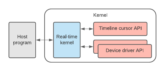
Fig. 4. A schematic overview of a host program a kernel with access to APIs

for the timeline cursor and device drivers.

For the RTIO system to operate proper ly, the slack (i.e.

the difference between the timeline cursor and the RTIO

counter) must be positive. Postin g an event with negative slack

translates to changing the state of a device in the past, which

is not possible. Doing so will result in an underﬂow exception.

Kernels normally start their pr ogram by synchron iz ing the

timeline cursor to the RTIO counter and incrementing the

timeline cursor with a ﬁxed value of 125 × 10

MU to ensure

positive slack at the start of the program.

B. Software

The ARTIQ software environment is Python-based a nd

programs that run on the system are called experiments. An

experiment consists o f Python code that runs on the host and

can additionally contain kernel functions that run on the core

device. Kernel functions are written in the ARTIQ domain-

speciﬁc language (DSL) which is a subset of the Python lan-

guage. Inside kernels, programmers have access to additional

functions to manipulate the timeline cursor, post events, and

read input buffers. The latter two are norma lly not directly

used by progr a mmers as these functions are encapsulated in

device drivers. Such device drivers provide an application

programming interface (API) to translate functional device

behavior (e.g. switch off a digital output pin) to low-level

events. A schematic overview of a ho st program and a kernel

with access to APIs for the timeline cursor and device d rivers

is shown in Figure 4.

When the host calls a kernel function , the ARTIQ compiler

assembles a kernel binar y at ru ntime which is then uploaded

to and executed by the core device. Variables from the host

environm e nt th a t are accessed in a kernel will be compiled

into the binary. During kernel execution, th e host will handle

any (a)synchronous remote procedure calls (RPCs) initiated by

the kernel. Once the kernel is ﬁnished executing, the context

switches back to the host, an d any variables modiﬁed in the

kernel are synchronized with the host environm ent before

the experiment resumes executing on the host. As a result,

the context switch between host and kernel co de is almost

seamless from a programmer’s perspective.

IV. SIMULATION

Our goal is to enable the simulation of re a l-time control

software for software te sting and veriﬁcation. A simulator

should integrate into the existing ARTIQ environment, sim-

ulate kernel execution, and simulate any interactions between

the host environment and the kernel as described in Section III.

The simulator should be fast enough to test comple te experi-

ments within a reasonable time. No real-time control hardware

should be requ ired to run simulations, only a mod el of the

hardware listing the available devices. Hardware/software co-

simulation for embedded systems is not new, and existing

work proposes various techniques and approaches for such

simulations [ 16], [17]. At the most detailed level, we ﬁnd

cycle-accurate simulations, such as [18], [19], [21], that take

the same binary as the real system and simulate the compo-

nents and registers of the microarchitecture in great detail.

Such simulations require highly detailed models making them

inﬂexible and potentially time-consuming to develop. Cycle-

accurate simu la tors are extremely detailed and accur ate but are

also slow. It is not our goal to do perform ance analysis on the

ARTIQ microarchitecture, an d we do not need such a level of

detail. Since our target is software testing and not hardware

performance analysis, we will focus on API simulation. An

API simulation cross-com piles the target progr am to a simu-

lator that implements the same API as the target system. The

simulator r equires no execution model of the hardware and

can therefore be fast. Based on our requirements, we decide

to target functional simulation of kernels and real-time devices

using API simulation. Timeline cursor man ipulations will be

simulated at the A PI level. Real-time devices are simulated

at their driver API level, and functional behavior will be

based o n a simpliﬁed device mo del. Hence, we will replace

the timeline cursor API and the device driver APIs shown in

Figure 4 with calls to our simulation infrastructure. The state

of the RTI O counter and RTIO engine are not simulated, which

would require the use of a cycle-accurate simulator. Instead,

we estimate the value of the RTIO counter when synchr onizing

the timeline cursor with the RTIO counter.

For simulation o f real-time kernels, we will need to cover

classical constructs (i.e. the CPU), the timeline cursor, the

event timeline, and input buffers. Since both the host code

and the classical co nstructs of the kerne ls are valid Python

code, we dec ided to use the host Python process to simulate

kernels. Hence, our simulator is implemented in Python a nd

all components in Figure 4 will be executed by the Python

interpreter. Using the same Python process will also instantly

implement host-kernel variable synchronization and ha ndling

of RPCs. We decided to split the simulation of the remaining

components into two parts: time and signals. The time com-

ponen t covers the simulation of the time line cursor, and the

signals component covers the simulation of the event timeline

and input buffers. Figure 5 shows a schematic overview of the

simulated components. In the remainder of this section, we

will cover time and signal simulation.

A. Time

A kernel can read and write the value of the timeline cursor

using the functions now_mu() and at_mu(t), respectively.

Additionally, the cursor can be moved relative from its current

Fig. 5. A schematic overview of the simulated microarchitectural components.

position using the functions delay_mu(d) and delay(d).

The latter func tion is used with a de lay time expressed in

seconds instead of MU. Since the delay in seconds is converted

to a delay in MU, the delay(d) function is not further

discussed. Fun ctions used to modify the timeline cursor behave

differently depending on the timing context in which they are

used. There are two timing con texts, sequential and parallel,

which are used as regular Python context managers using the

with statement. The two contexts are used to specify if a

set of RTIO operations should be executed sequentially or in

parallel. The contexts can be nested ar bitrarily, and by default,

every function starts in a sequential context. As a result, the

timeline cursor simulation will have to adapt based on the

current timing context.

In a sequential context, any modiﬁcation to the timelin e

cursor is interpreted as a seque nce of operations. Hence, two

successive delays with duration d

and d

is equal to one

delay with duration d

. Any call to at_mu(t) is a pplied

instantly. Modiﬁca tions to the timeline cursor in a parallel

context are postponed such that operations in the context can

be interpreted as parallel. Wh en the program exits the parallel

context, the timeline cursor will be moved f orward by the

duration of the long e st positive delay. If a para llel context

containing delays with duration d

, . . . , d

is entered with

the timeline cur sor at t

start

, the timeline curso r will be set to

start

+max (0, d

, . . . , d

) when the context exits. In a parallel

context, calls to at_mu(t) with value t

new

are interpreted as

delays with duratio n t

new

− t

start

We simulate the time line cursor using a stack of simulation

contexts that represen t the nested timin g contexts. The ap-

propriate simulation context is pushed on and po pped off the

stack wh e n a timing context is entered and exited, respec tively.

Each simulation context holds a current time t

current

and a

duration t

duration

variable in MU. When pushed to the stack,

current

is inherited fr om the simulation context currently at th e

top of the stack while t

duration

is always initialized to zero.

When a simulation context is popped off the stack, t

duration

is propagated to the underlying simulation context as a delay.

There is a sequential and a parallel simulation context availab le

and when the simulation starts, the stack is initialized with a

sequential simulation context with t

current

= 0. At any time,

interactions with the timeline cursor are handled by the context

at the top of the stack. now_mu() always returns t

current

while calls to delay_mu(d) are handled differently by the

sequential and parallel simulation context. For a sequential

simulation context, a delay with duration d will in crement

current

and t

duration

by d while for a parallel simulation context,

current

is not changed and t

duration

= max (t

duration

, d). For both

simulation contexts, calls to at_mu(t) with value t

new

are

converted to delays with duration t

new

− t

start

. The described

system using the stack of simulation contexts accu rately sim-

ulates the behavior of the timeline cursor.

For correct synchr onization of the timeline cursor to the

RTIO counter, we keep track of a timeline horizon which is

essentially an estimation RTIO counter state. For a simulation

with events a t timestamps t

, . . . , t

, the timeline horizon is

deﬁned as max (t

cursor

, t

, . . . , t

) where t

cursor

is the current

position of the timeline cursor. Whe n we synchronize the

timeline cursor to the RTIO counter, we ﬁrst set the po sition

of the timeline cursor to the position of the timeline horizon

before inserting a delay of 125 × 10

MU. Using the timeline

horizon for sync hronization is necessary to simulate code with

negative delay s corr ectly. Negative delays a re commo nly used

to compensate for latencies of physical equipment.

B. Sig nals

For signal simulation, we need to simulate the event timeline

and the input buffers. Interaction s with the event timeline

and input buffers happen through device drivers. We simulate

device drivers on an API level, and each driver simulates the

signals and state of a device based on a simpliﬁed model.

Signals will be simulated on a functional level, for examp le ,

frequency an d phase for a direct digital synthesis (DDS) chip

and a binary state for a digital output. To enable signal

simulation, we will capture all function calls to drivers by

replacing each device driver with a matching simulation driver.

During initialization, each simulation driver obtains one or

more nam e d signal objects corresponding to the state of the

device. Each time a driver fun c tion is called to change the

state of th e device, the dr iver will push new values to the

appropriate signal objects. Pushing a new value to a signal

object will cause an event to be c reated at th e current position

of the timeline cur sor. Each signal object stores its events

and therefore possesses a part of the complete event timeline

of the system. If two events for a single signal have the

same timestamp, the latest event overwrites the existing event.

Additionally, the simulation driver can keep a n internal state

and perf orm any additional processing for proper signal and

time simulation.

To test real-time control software, we must have the ability

to read the value of a signal at any given timestamp. To pull

the value of a signa l at a speciﬁc timestamp, we search for the

event with the highest timestamp that is less or equal to the

timestamp of interest. The value of that event will represent

the value of the signal at the given timestamp. If no event is

found, the signal has not been set, and its value is unknown.

The last component that must be simulated is the input

buffers. Values in these buffers origina te from events with

return values, such as sampling the value of a digital input

device. For software testing, return values from input devices

must be conﬁgurable by a test case. For th at purpose, we

introdu ce input signals that describe the state of a hypothetical

device that generates the input signal observed by a device.

Just as o utput signals, input signals a re obtained by the device

drivers during initialization, for example, an input probability

signal for a digital input device. When the simulation driver

is called to sample the input value, the driver p ulls the current

value of the input p robability signal and uses it to generate

a return value. The return value is stored in the input buffer

that is part of the simulatio n driver. Once the actual sampled

value is requested from the driver, th e value is taken from the

buffer an d retu rned. Each input device has input signals that

match the level of its functionality, such as input voltage for an

analog-to-digital converter (ADC) and input frequency for a

digital edge counter. During software testing, input signals can

be conﬁg ured using the same pu sh/pull infrastructure used for

output signals. This allows input signals to be adjusted using

the same event timeline as output signals.

C. Implementation

We have implemented a simulation platform for ARTIQ

based on the propo sed methodologies for time and signal sim-

ulation. The simulator is part of our open-source library Duke

ARTIQ extensions (DAX) [35] which in tegrate s tightly with

the ARTIQ open-so urce software environment. The integration

entry point for the DAX simulator is the device database

(DDB), a c entral ﬁle in every ARTIQ proje ct that deﬁnes

the list of availab le real-time devices and th eir correspond ing

drivers. To enable simu la tion, users m ake a small modiﬁcation

that allows the DAX simulation infra structure to mutate the

DDB bef ore ARTIQ reads it at the start of an experiment.

During DDB mutation, all device drivers are replaced by

matching simulation drivers, a nd an extra simulation conﬁg-

uration device is inserted into the DDB. When the driver for

the core d evice is loaded in an experiment, the core device

simulation driver will be loaded, w hich in turn loads the driver

for the simulation conﬁguration device. The DAX simulation

infrastructure is loaded during initialization of the simulation

conﬁguration device, which includes the setup of a time and a

signal manager. Any other simulation drivers that are loaded

will request their signal objects from the signal manager.

When the expe riment runs and a kernel function is called,

the core device driver is requested to compile the kernel and

execute it on the core device. Instead, the simulation driver

for the core device will ju st run the kernel function inside a

sequential time context using the current Python process. Any

interactions with the timeline cursor or time context APIs are

forwarded to the time manage r for simulation while simulatio n

drivers will perform all the signal simulations. Events for

each signa l are stored in a sorted dictionary based on their

timestamps, and binary search algorithms are used to push

and pull events.

We integrated our simulation platform with the standard

Python unit test framework such that users can r un tests fo r

real-time control software using existing testing environments.

The DAX unit test base class, which inherits the standard

Python unit test class, provides functions to push, pull, and test

signal values at any timeline cursor position. Existing too ls for

step debugging, automated testing, and continuous integration

will allow real-time control software to be tested to the same

level as any other production-level software project.

D. Limitations

Functional simulation of kernels at the API level is fast

and especially useful for testing and veriﬁcation of real-time

control software, but it also has limitations. Without simulation

of the RTIO counter and the RTIO engine, slack can not be

reliably simulated. As a result, API simulation can not accu-

rately predict und erﬂow exceptions. A low-level and cycle-

accurate micro architectural simulation would be required to

simulate slack. Such simulators are much slower and are not

convenient for software testing and veriﬁcation at the level

discussed in this paper.

Some limitations are speciﬁc to our implem entation of the

simulation infrastru cture. We use the running Python process

to execute kernels, but th e ARTIQ DSL only supports a

subset of the Python language. He nce, the simulation is more

permissive than the ARTIQ compiler. We can mitigate this

issue by compiling kernels before simulation. By default, the

DA X simulator does not compile kernels to run simulations

faster.

Host-kernel attribute synchronizatio n also behaves differ-

ently in simulation. When running on a co re device, the

ARTIQ environment synchronizes host variables modiﬁed in a

kernel wh en the kernel ﬁnished executing (see Section III-B).

During simulation, attributes are continuously synchronize d

due to the use of a single Python process for host and kernel

code. The behavior of the simulator could be different when

a kernel modiﬁes the same variable used by an RPC function

it calls. Su ch code would have confusing semantics to start

with, and we have not encountered any such code.

The model of the parallel timing context descr ibed in Sec-

tion IV-A differs slightly from the timing model imple mented

in the ARTIQ compiler. The DAX simula tor propagates the

parallel semantics until a sequential context is entered (deep

parallel) while the ARTIQ compiler only propa gates the par-

allel semantics to top-level statements in the context (shallow

parallel). Kernel code that potentially behaves differently with

deep and shallow parallel semantics can be detected using

abstract syntax tree (AST) analysis. We have developed a

separate tool [36] that ﬂags such kernel code.

V. EVALUATION

To evaluate the p erformance of the DAX simulation plat-

form, we measured its kernel execution time and compared

Label Experiment

mw freq Microwave frequency scan

rabi Microwave Rabi frequency scan

mw ramsey Microwave Ramsey scan

mw gate Microwave repeated gate scan

gco

freq Global co-propagating frequency scan

gco rabi Global co-propagating Rabi frequency scan

gco ramsey Global co-propagating Ramsey scan

ico freq Individual co-propagating frequency scan

ico

ttime Individual co-propagating time scan

state init Qubit state initialization scan

tickle Tickle scan

direct rb Direct randomized benchmarking

gst Gate set tomography

sqst Single-qubit state tomography

TABLE I

LI ST OF EXPERIMENTS US ED F OR THE EVALUATION.

it to the execution time on hardware. We used two experi-

mental tr apped-io n quantum processors for our evaluation, the

software-tailored architecture for quantum co-design (STAQ)

system [8] and the red chamber (RC) system [37] . Both

systems are con trolled by an ARTIQ co ntrol system, but

STAQ uses a core device based on the Kasli 2.0 contr oller

[15] while RC uses a KC705-based controller [38]. Besides

the different real-time control systems and devices, the main

difference between these two setups is that STAQ is at

cryoge nic temperatu res while RC is at room temperature. We

chose 14 commonly used exp e riments with a single kernel for

the STAQ system. The set of experiments, listed in Table I,

contains 11 scanning-type experiments used for calibration and

three benc hmarking experimen ts including, Direct randomized

benchm arking (RB) [39]–[41], gate set tomography (GST)

[42], and single-qubit state tomography ( SQST) [43]. Both

systems use modular real-tim e control software developed with

the DAX modular software framework [44], and parts of the

system-speciﬁc control software are available in the DAX-zoo

repository [45]. The three benchmark experiments are portable

and can also run on RC while the four microwave (MW)

calibration experiments have an equivalent implementation

for the RC system. All scanning-type experim ents scan over

20 points and take 100 samples per point. Direct RB is

performed with circuit lengths startin g at 1 and scaling up

exponentially to 16. For each circuit length, we benchmark

ten different circuits with 100 samples for each circuit. The

GST benchmarks are performed with a total of 523 different

circuits based on our germs, taking 100 samples per circuit.

Finally, SQST is perfo rmed with a grid of 5 times 10 angles

taking 100 samples for each point.

For our evaluation, we r un the experime nts for both sys-

tems o n a Kasli 2.0 controller. The RC software can run

on an appropria te ly conﬁgured Kasli controller by replacing

the DDB. All calibration experiments are executed with and

without buffering. Bu ffering allows the real-time co ntrol soft-

ware to schedule the operations for the next samples w hile

the incoming data of earlier samples are kept temporally in

hardware buffers. ARTIQ supports such hardware buffers,

mw_freq

mw_rabi

mw_ramsey

mw_gate

gco_freq

gco_rabi

gco_ramsey

ico_freq

ico_time

state_init

tickle

direct_rb

gst

sqst

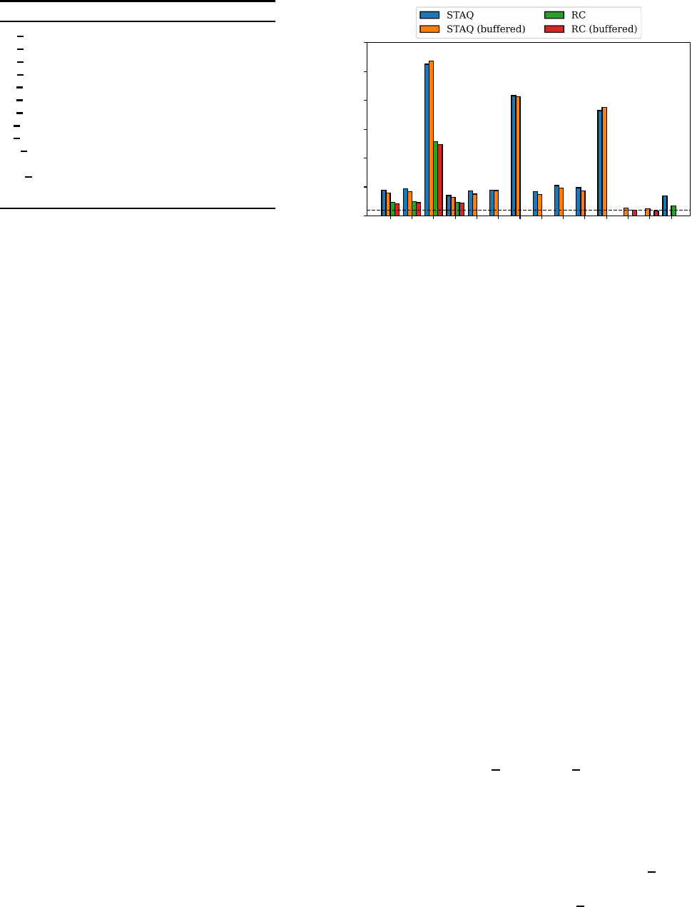
Speedup

Fig. 6. Kernel execution time speedup for our simulator relative to the

execution time on a core device.

but the real-time software must be designed appropriately to

utilize them. Buffering can further increase the thr oughput

and performance of kernels by reducing stalling time at the

cost o f incre a sed latency between receiving and processing

input events. None of the experiments are sensitive to the

increased latency and will beneﬁt from increased throughput.

We conﬁgure a buffer size of 16 samples, which should be

large enough to get th e maximum pe rforman ce gain achievable

with buffering. The Direct RB and GST exp eriments are

always buffered with a ﬁxed buffer size of 1 and SQST is

always unbuffered. The kernel execution time is measured with

nanosecond precision using the real-time clock available in

the Kasli controller. We then run the same experiments u sin g

our DAX simulation platform on a computer equipped with

an AMD Ryzen 7 3700X CPU and 32 GB of memory. The

computer runs on Ubuntu 20.04 LTS, and the execution time

of the kernel simulation is measu red in nanosecon ds using

the standard Python time library. All experime nts run ﬁve

times on hardware and ﬁve times in simulation to take the

average simulation time. Our measurements are performed

using ARTIQ version 6.7659.c6a7b8a8 and the results are

presented in Figure 6.

The results in Figure 6 show that simulation speeds up

execution up to 2 6.8 times with an average speedup of 6.9

times. Especially the mw

ramsey, gco ramsey, and tickle

experiments achieve large sp e edups. The exceptional speedup

for these experiments is caused by the long delays th at are

part of the experiment. The core device waits for these delays

before the kernel ﬁnishes execution, while the simulator only

simulates the passing o f time but does not wait for it. The

experiments that show the least speedup are the direct

rb and

gst experiments. For STAQ, both experimen ts only yield a 1.3

times speedup, while for RC, the direct

rb experimen t has

no speedup and the gst experiment is slower with a speedup

of 0.8 times. The limited speedup of these two experiments

is caused by short delays and a high number of operations,

which results in a h igh event density. As a result, the sim ulator

must process many events while the experiment has a relatively

short execution time on hardware. In general, we could state

that the execution time on hardware t

hardware

is m ostly limited

by the length of delays inser ted during the experiment. These

delays sum up to the total length of the timeline and therefore

the duration of the experiment when running on hardware.

The execution time of the simulator t

sim

is not much affe cted

by d elays and instead is mostly limited by the total number

of events present in the exp e riment. We know that speedup

is deﬁne d as S = t

hardware

sim

. Roughly speaking, we can

derive that the to ta l duration of an experiment is proportional

to speedup while the total number of events is inversely

proportional to speedup.

We can see from Figure 6 tha t th e experiments running

on the RC system always yield lower speedup compared to

the same experiment running on STAQ. The different results

are caused by differences in the control for the cooling and

pumping pro cedures. Both procedures are executed by a ll

experiments at the star t of ea ch sample. STAQ uses three

digital outputs and one DDS while RC h a s additional features

and uses ﬁve digital outputs and a DDS. As a result, RC

inserts more events for each cooling and pumping procedu re.

Additionally, STAQ uses a constant DDS frequency for both

proced ures while RC uses a different frequency for each pro ce-

dure which adds two additional DDS conﬁguration events for

each sample. Hence, the total number of events for RC exper-

iments is higher than for STAQ which reduces the speedup.

The additional DDS operations also inser t extra delays into

the experime nt, but these delay s do not c ompensate for the

increased number of events. Figure 6 also shows buffered

experiments tend to have slightly less speedup compared to

their unbuffered counterparts. Buffering can reduce the execu-

tion time overhead of exper iments resulting in faster execution

on hardware. The total number of events per experiment is

not affected by buffering. The result is a reduced speedup for

experiments with buffering. The reduction in execution time

by buffering is limited though due to the highly optimized

control software.

In addition to speedup, we have also measured the timing

accuracy of the simulated timeline cursor compared to execu-

tion on the core device. High timing accuracy is not a speciﬁc

requirement for correct functional simulation, but a simulator

with high timing accuracy could be used for estimating the

timing of experiments. The timeline cursor simulation is ac-

curate, but variable delays and inaccurate d e la ys in simulated

device drivers can still introduce errors. Variable delays mainly

occur whe n the timeline cursor is synchroniz e d with the RTIO

counter. Such synchronization is performed at least on ce at

the star t of the experiment (see Section III-A) but can also

occur at other mome nts. We simulate the synchro nization

of the timeline cursor using a timeline horizon and insert

an additional delay of 125 × 10

MU. We would like to

emphasize that the presence of a variable delay indicates that

the relative timing between th e events before and after the

delay is not re levant, and any variation will not negatively

mw_freq

mw_rabi

mw_ramsey

mw_gate

gco_freq

gco_rabi

gco_ramsey

ico_freq

ico_time

state_init

tickle

direct_rb

gst

sqst

0.15

0.10

0.05

0.00

0.05

0.10

Relative error

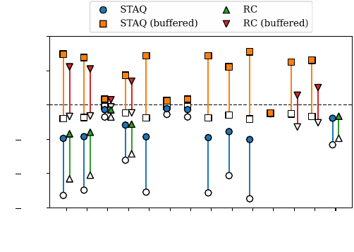
Fig. 7. The error of the simulated timeline cursor relative to the timeline

cursor of the core device. The ﬁlled markers represent the regular conﬁguration

while empty markers represent the optimistic conﬁguration.

impact the functionality o f the experiment or the simulation.

Hence, simulating timeline cursor synchronization with a

timeline horizon is sufﬁcient for correct functional simulation.

A variable delay can also occur when an experiment needs

to wait for an input event that occ urs at an unpredictable

time, though none of the experim ents in Table I contain such

constructions. Inaccu rate delays in simulated device drivers

are often cau sed by a simpliﬁed timing model of the device

driver. In practically all cases with inaccuracy, the simulated

driver inserts less delay than the actu a l driver.

To measure the timing accuracy of the simulated timeline

cursor, we store the value of the timeline cursor after the ﬁrst

synchro nization with the RTIO counter and at the end of the

experiment. The difference between the two values represents

the total length of the event timeline in MU. We run the

simulations with two conﬁgurations: regular and optimistic.

When the timeline cursor is synchronized with the RTIO

counter, our simulator inserts a ﬁxed delay of 125 × 10

and

0 MU for the regular an d optimistic conﬁg uration, respectively.

We measured the event timeline length on the core device

and with the two simulation conﬁg urations for a ll experiments

listed in Table I using the STAQ and RC system. For e ach

combination of system, experiment, and conﬁguration, we

calculate the relative er ror of the simulation which is deﬁned

as (t

sim

− t

exe

)/t

exe

where t

exe

and t

sim

are th e measured event

timeline lengths on the core device and during simulation,

respectively. The results for are shown in Figure 7 and are

also listed in Table II and III.

The results in Figure 7 show the error of the simulated time-

line cursor relative to the timeline cursor of the core device.

The regular and optimistic conﬁgurations are represented by

the ﬁlled and empty markers, respectively. When comparing

the re sults of the two different conﬁgurations, we see that the

optimistic conﬁguration always estimates a shor ter timeline

length, which is expected. If we only look at the results fo r the

optimistic conﬁguration, we see that all have a relative error

Experiment STAQ STAQ (buffered)

Regular Optimistic Regular Optimistic

mw freq -4.9% -13.2% 7.4% -2.0%

mw rabi -4.6% -12.4% 6.9% -1.8%

mw ramsey -0.7% -1.8% 0.9% -0.2%

gate -2.9% -8.0% 4.4% -1.2%

gco freq -4.6% -12.7% 7.2% -1.9%

gco rabi -0.5% -1.4% 0.6% -0.2%

gco ramsey -0.7% -1.7% 0.9% -0.2%

ico

freq -4.8% -12.8% 7.2% -1.9%

ico time -3.9% -10.3% 5.6% -1.5%

state init -5.0% -13.7% 7.8% -2.0%

tickle -1.2% -1.3% -1.2% -1.3%

direct

rb 6.2% -1.3%

gst 6.5% -1.7%

sqst -1.9% -5.8%

TABLE II

THE ERROR OF THE S IMULATED TIMELINE CURSOR RELATIVE TO THE

TIMELINE CURSOR OF THE CORE DEVICE FOR STAQ .

Experiment RC RC (buffered)

Regular Optimistic Regular Optimistic

mw freq -4.2% -10.8% 5.6% -1.7%

mw rabi -4.0% -10.2% 5.3% -1.6%

ramsey -0.7% -1.7% 0.8% -0.3%

mw gate -2.8% -7.1% 3.5% -1.1%

direct rb 1.4% -3.2%

gst 2.5% -2.6%

sqst -1.6% -4.9%

TABLE III

THE ERROR OF THE S IMULATED TIMELINE CURSOR RELATIVE TO THE

TIMELINE CURSOR OF THE CORE DEVI CE F OR RC.

lower or equa l to 0.0. The optimistic conﬁguration represents

the lower-bound execution time where variable delays a re

always zero. When ru nning on a ctual ha rdware, variable delays

are not always zero, and as a result, the optimistic conﬁgura-

tion underestimates the timeline length. We also noticed that

all un buffered results with regular conﬁguration h ave a relative

error lower or equal to 0.0. When running on hard ware w ithout

buffers, the system has negative slack after each sample,

and timeline synchronizations will insert de la ys larger than

125 × 10

MU. The regular conﬁguration underestimates the

length of the variable delay and therefore underestimates the

total timeline length. Regardless, the estimation of the regular

conﬁguration is better than that of the optimistic conﬁgu-

ration for unbuffered experiments. The opposite is true for

buffered experiments. Buffering reduces the length o f variable

delays caused by timeline synchro nizations by maintaining

slack between samples. The regula r conﬁguration is often too

pessimistic for buffered exp e riments and the e stima tion of the

optimistic conﬁgur ation is better most of the time.

We noticed two other trends in Figure 7 that relate to

the total timeline length of experiments. First, the results of

some experiments have little spread, in particular mw

ramsey,

gco

rabi, gco ramsey, and tickle. These are all calibration

experiments with relatively lo ng delays and long total timeline

lengths. The long timeline length combined with the limited

sources of errors (i.e. low density of variable delays and

events) results in a small relative er ror and therefore, a small

spread between different conﬁgurations. Second, the results

of the RC system tend to be closer to 0.0 than the equivalent

STAQ results. We already mentioned tha t due to differences

in the cooling and pu mping pro cedures, the RC system in-

serts more events for each sample of the experiment. These

additional events also insert extra delays into the experiment.

As a result, the total timeline length of RC experiments are

on average 28. 1% longer compared to their STAQ equivalents.

Again, the increased timeline length with no additional sources

of errors reduces the relative error.

Overall, th e average relative error for the regular conﬁg-

uration is 3.6%, and for the optimistic conﬁguration, the

average relative error is 4.4%. Based on our analysis of the

regular and optimistic conﬁgurations, we concluded that the

timeline length of buffered and unbuffered experiments ar e

better e stima te d by the regular and optimistic conﬁgurations,

respectively. When choosing the optimistic conﬁguration for

buffered experiments and the regular conﬁguration for un-

buffered experiments, the resulting average relative er ror is

reduced to 2.1%, leading to an average a c curacy of 97.9%. We

can conclude that even in the presence of variable delays and

simulated device dr ivers with simpliﬁed timing mod els, the

position of the timeline cursor is simulated with high accuracy

when choosing the appropriate conﬁguration.

VI. CONCLUSION

We have presented a functional simulation platform for

real-time control software that ena bles software testing and

veriﬁcation. To simplify testing and veriﬁcation, timeline ma-

nipulations and d evice drivers are simulated on the application

programming interface (API) level. Our simulation platform

accurately simulates a timeline cursor using a stack while

the event timeline is sim ulated using signals and events.

Input signals are also simulated on a f unctional level and

use the same interactive signal and event infrastructure used

for outpu t signals. We implemented a simulator based on the

proposed concepts, which is part of our open-source library

Duke A RTIQ extensions (DAX). Our simulator integrates

tightly into the advanced rea l-time infrastructure for quantum

physics (ARTIQ) environm ent and is capable of simulating

real-time kernels and host-kernel intera ctions. We integrated

our simulator with the standard Python unit test frameworks

such that real-time con trol so ftware can be tested using ex-

isting tools for step debugging, unit testing, and continuous

integration. Compar e d to kernel execution on the core device,

kernel simulation is 6.9 times faster on average. Even with

the presence of variable delays and simpliﬁed timing models

for device drivers, the position of the timeline cursor is

simulated with an average accuracy of 97.9% when choosing

the appropriate conﬁguration.

ACKNOWLEDGMENT

This work is fund e d by EPiQC, an NSF Expeditions in

Computing (1832377), the Ofﬁce of the Director of National

Intelligence - Intelligence Advanced Research Projects Activ-

ity throu gh an ArmyResearch Ofﬁce contract (W911NF-16-1-

0082) and the NSF STAQ project (1818914).

REFERENCES

[1] F. Arute, K. Arya, R. Babbush, et al.,

“Quantum supremacy using a programmable

superconducting processor,” Nature, vol. 574, no. 7779,

pp. 505–510, Oct. 2019, ISSN: 1476-4687. DOI:

10.1038/s41586-019-1666-5. [Online]. Available:

https://doi.org/1 0.1038/s41586-019-1666-5.

[2] C. Ryan-Anderson, J. G. Bohnet, K. Lee,

et al., “Realization of real-time fault-tolerant

quantum error correction,” Phys. Rev. X,

vol. 11, p. 041 058, 4 Dec. 2021. DOI:

10.1103/PhysRevX.11.041058. [Online]. Available:

https://link.aps.org/doi/10.1103/PhysRevX.11.041058.

[3] L. Postler, S. Heußen, I. Pog orelov, et al., Demon-

stration o f fault-to le rant universal quantum gate oper-

ations, 2021. DOI: 10.48550/ARXIV.2111.12654. [On-

line]. Available: https://arxiv.org/abs/2111.1265 4.

[4] Y. Wang, Y. Li, Z.-q. Yin, et al., “16-qubit ibm uni-

versal quantum compute r can be fully entan gled,” npj

Quantum information, vol. 4, no. 1, pp. 1–6, 2018.

[5] I. Pogorelov, T. Feldker, C. D. Marciniak, et al.,

“Compact ion-trap q uantum computing de monstrator,”

PRX Quantu m , vol. 2, p. 020 343, 2 Jun. 2021. DOI:

10.1103/PRXQuantum .2.020343. [Online]. Available:

https://link.aps.org/doi/10.1103/PRXQuantum.2.020343.

[6] R. Acharya, I. Aleiner, R. A llen, et al., Suppress-

ing quantum errors by scaling a surface code logical

qubit, 2022. DOI: 10.48550/ARXIV.2207.06431. [On-

line]. Available: https://arxiv.org/abs/2207.0643 1.

[7] G. Pagano, A. Bapat, P. Becker, et al., “A quantum

approximate optimization algorithm in a tra pped-ion

quantum simulator,” en, Oct. 2020. [Online]. Available:

https://tsapps.nist.gov/p ublication/get

pdf.cfm?pub id=928237.

[8] J. Kim, T. Chen, J. Whitlow, et al., “Hardware design o f

a trapped-ion quantum computer for software-tailored

architecture for qu antum co-design (staq) project,”

in Quantum 2.0, Optical Society of America, 2020,

QM6A–2.

[9] M. Blok, V. Ramasesh, T. Schuster, et al., “Quantum

informa tion scrambling in a superconducting qutrit pro-

cessor,” arXiv preprint arXiv:2003.03307, 2020.

[10] S. Bourdeauducq, R. J¨ordens, P. Zotov, et

al., Artiq 1.0, version 1.0, May 2016. DOI:

10.5281/zenodo.51303. [Online]. Available:

https://doi.org/1 0.5281/zenodo.51303.

[11] V. Negnevitsky, “Feedback-stabilised quantum states in

a mixed-species ion system,” Ph.D. dissertation, ETH

Zurich, 2018.

[12] P. Maunz, J. Mizrahi, and J. Goldberg, Ioncontrol

v. 1.0, version 00, Jul. 2016. [Online]. Available:

https://www.osti.gov/biblio/1326630.

[13] X. Fu, L. Riesebos, M. A. Rol, et al., “Eqasm: An ex-

ecutable quantum instruction set architecture,” in 2 019

IEEE International S ymposium on High Performance

Computer Architecture (HPCA), 2019, pp. 224–237.

DOI: 10.1109/HPCA.2019.00040.

[14] C. A. Ryan, B. R. Johnson, D. Rist`e, et al., “Hardware

for dynamic quantum computing,” Review of Scientiﬁc

Instruments, vol. 88, no. 10, p. 104 703, 2017.

[15] G. Ka sprowicz, P. Kulik, M. Gaska, et al., “Ar tiq

and sinara: Open software and hardware stacks for

quantum physics,” in OSA Quantum 2.0 Conference,

Optical Society of America, 2020, QTu8 B.14. DOI:

10.1364/QUANT U M.2020.QTu8B.14. [Online]. Avail-

able: http://www.osapublishing.org/abstract.cfm?URI=QUANTUM-2020-QTu8B.14.

[16] J. Rowson, “Hardware/software co-simu la tion,” in 31st

Design Automation Conference, 19 94, pp. 439–440.

DOI: 10.1109/DAC.1994.204143.

[17] K. Hines and G. Borriello , “Dynamic communica tion

models in embedded system co-simulation,” in Proceed-

ings of the 34 th Annual Design Automation Conference,

ser. DAC ’97 , Anah eim, California, USA: Association

for Com puting Ma chinery, 1997 , pp. 395–400, ISBN:

0897919203. DOI: 10.1145/266021.266178. [Online].

Available: https://doi.org/10 .1145/266021.266178.

[18] J. Lowe-Power, A. M. Ahmad, A. Akram, et

al., The gem5 simulator: Version 20.0+, 2020.

DOI: 10.48550/ARXIV. 2007.03152. [Online]. Avail-

able: https://arxiv.org/abs/2007.03152.

[19] P. R. Panda, “ Systemc: A modeling platform supporting

multiple design abstractions,” in Proceedings of the

14th Internationa l Sy m posium on Systems Synthesis,

ser. ISSS ’01, Montr´eal, P.Q., Canada: Association

for Computing Mac hinery, 2001, pp. 75–80, ISBN:

1581134185. DOI: 10.1145/500001.500018. [Online].

Available: https://doi.org/10 .1145/500001.500018.

[20] “Ieee standard for standa rd systemc language ref-

erence manual,” IEEE Std 1666-2011 (Revision

of IEEE Std 1666-2005), pp. 1–638, 2012. DOI:

10.1109/IEEESTD.2012.6134619.

[21] J. Bachrac h, H. Vo, B. Richards, et al., “ Ch isel: Con-

structing hardware in a scala embedded language,”

in DAC Design Automation Co nference 2012, 2012,

pp. 1212–1221. DOI: 10.1145/2228360.2228584.

[22] C. H e lmstetter and V. Joloboff, “Simsoc: A systemc

tlm integrated iss fo r full system simulation,” in APC-

CAS 2008 - 2008 IEEE Asia Paciﬁc Conference on

Circuits and Systems, 2008, pp. 1759–1762. DOI:

10.1109/APCCAS.2008. 4746381.

[23] C. Erbas, A. D. Pimentel, M. Thompson, et al., “A

framework for system-level modeling and simulation

of embedded systems architectures,” EURASIP Journal

on E m bedded Systems, vol. 2007, no. 1, p. 082 12 3, Jul.

2007, ISSN: 1687-3963. DOI: 10.1155/2007/82123. [On-

line]. Available: https://doi.org/10.1155/2007/82123.

[24] A. Pimentel, C. Erbas, and S. Polstra, “A systematic

approa c h to exploring embedded system architec tures

at multiple abstraction levels,” IEEE Transactions on

Computers, vol. 55, no. 2, pp. 99–112, 2006. DOI:

10.1109/TC.2006.16.

[25] G. Li, Y. Din g, and Y. Xie, “Sanq: A simulation frame-

work for architecting noisy intermediate-scale quantum

computing system,” arXiv preprint arXiv:1904.115 90,

2019.

[26] X. Fu, J. Yu, X. Su, et al., “Quingo: A pro-

gramming fr a mework for heterogeneous quantum-

classical computing with nisq features,” arXiv preprint

arXiv:2009.01686, 2020.

[27] L. Riesebos, X. Fu, S. Varsamopoulos, et al.,

“Pauli frames for quantum computer architectures,”

in Proceedings of the 54th Annual Design

Automation Conference 2 017, ser. DAC ’17,

Austin, TX, USA: Association for Computin g

Machinery, 2017, ISBN: 9781450349277. DOI:

10.1145/306 1639.3062300. [Online]. Available:

https://doi.org/1 0.1145/3061639.3062300.

[28] L. Riesebos, X. Fu, A . Moue ddenne, et al.,

“Quantum accelerated computer architectures,” in

2019 IEEE International Symposium on Circuits

and Systems (ISCAS), 2019, pp. 1–4. DOI:

10.1109/ISCAS.2019.8702488.

[29] K. M . Svore, A. Geller, M. Troyer, et al. , “Q#: Enabling

scalable quantum computing and development with a

high-level domain -speciﬁc language,” arXiv preprint

arXiv:1803.00652, 2018.

[30] T. Nguyen, A. Santana, T. Kharazi, et al., “Extending

c++ for heterogeneous quantum-classical computing,”

arXiv preprint arXiv:201 0.03935, 2020.

[31] R. S. Smith , M. J. Curtis, and W. J. Zeng, “A practical

quantum instruction set architecture,” arXiv preprint

arXiv:1608.03355, 2016.

[32] F. T. Chong, D. Franklin, and M. Martonosi, “Program-

ming languages and compiler design for realistic quan-

tum hardware,” Nature, vol. 549, no . 7671, pp. 180–187,

2017.

[33] J. E. Stone, D. Gohara, a nd G. Sh i, “Opencl: A parallel

programming standard for heterogeneous computing

systems,” Computing in science & engine ering, vol. 12,

no. 3, p. 66, 2010.

[34] X. Fu, M. A. Rol, C. C. Bultink, et al., “An

experimental microarchitecture for a superconduct-

ing quantum pro cessor,” in Proceedings of the

50th Annual IEEE/ACM International Symposium

on Microarchitecture, ser. MICRO-50 ’17, Cam-

bridge, Massachusetts: Association for Computing Ma-

chinery, 2017, pp. 813–825, ISBN: 9781 450349529.

DOI: 10.1145/3123939.3123952. [Online]. Available:

https://doi.org/1 0.1145/3123939.3123952.

[35] L. Riesebos, B. Bondurant, and K. R. Brown, Duke

artiq extensions (dax), 2021. [Online]. Available:

https://gitlab.com/duke-artiq/dax.

[36] L. Riesebos, Flake8 artiq plugin, 2020. [Onlin e]. Avail-

able: https://gitlab.com/duke-artiq/ﬂake8-artiq.

[37] Y. Wang, S. Crain, C. Fang, et al. , “High-ﬁdelity

two-qubit gates using a microelec tromechan ic a l-

system-based beam steering system for

individual qubit addressing,” Phys. Rev. Lett.,

vol. 125, p. 150 505, 15 Oct. 2020. DOI:

10.1103/PhysRevLett.125.150505. [Online]. Available:

https://link.aps.org/doi/10.1103/PhysRevLett.125.150505.

[38] Xilinx kc705. [Online]. Available:

https://www.xilinx. com/products/boards-and-kits/ek-k 7-kc705-g.html.

[39] E. Magesan, J. M. Gambetta, and J. Emerson, “Scal-

able and robust randomized benchm a rking of quantum

processes,” Physical review letters, vol. 106, no. 18,

p. 180 504, 2011.

[40] T. J. Proctor, A. Carignan -Dugas, K. Rudinger,

et al., “Direct randomized benchmarking

for mu ltiqubit devices,” P hys. Rev. Lett.,

vol. 123, p. 030 503, 3 Jul. 2019. DOI:

10.1103/PhysRevLett.123.030503. [Online]. Available:

https://link.aps.org/doi/10.1103/PhysRevLett.123.030503.

[41] J. M. Epstein, A. W. Cross, E. Magesan, et al., “Inves-

tigating the limits of randomized b e nchmark ing proto-

cols,” Physica l Review A, vol. 89, no. 6, p. 062 321,

2014.

[42] R. Blume-Kohout, J. K. Gamble, E. Nielsen, et

al., Robust, self-consistent, closed-form tomography of

quantum logic gates on a trapped ion qubit, 2013.

DOI: 10.4855 0/ARXIV.1310.4492. [Online]. Available:

https://arxiv.org/abs/1310.4492.

[43] R. Schmied, “Quantu m state tomography of a single

qubit: Comp a rison of methods,” Journal of Modern

Optics, vol. 63, no. 18, pp. 1744–17 58, 2016.

[44] L. Riesebos, B. Bondurant, J. Whitlow, et al., “Mod-

ular software for real-time quantum control systems,”

in 2022 IEEE International Conference on Quantum

Computing and Engin eering (QCE), 2022.

[45] Duke artiq extensions (dax) zoo, 2022. [Online]. Avail-

able: https://gitlab.com/duke-artiq/dax-zoo.