Determination of the Concentration of Atmospheric Gases By Gas Chromatography

McNair Scholars Research Journal McNair Scholars Research Journal

Volume 6 Article 6

2013

Determination of the Concentration of Atmospheric Gases By Gas Determination of the Concentration of Atmospheric Gases By Gas

Chromatography Chromatography

Chris Haskin

Eastern Michigan University

, [email protected]

Follow this and additional works at: https://commons.emich.edu/mcnair

Recommended Citation Recommended Citation

Haskin, Chris (2013) "Determination of the Concentration of Atmospheric Gases By Gas Chromatography,"

McNair Scholars Research Journal

: Vol. 6 , Article 6.

Available at: https://commons.emich.edu/mcnair/vol6/iss1/6

This Article is brought to you for free and open access by the McNair Scholars Program at DigitalCommons@EMU.

It has been accepted for inclusion in McNair Scholars Research Journal by an authorized editor of

DigitalCommons@EMU. For more information, please contact [email protected].

DETERMINATION OF THE CONCENTRATION

OF ATMOSPHERIC GASES BY

GAS CHROMATOGRAPHY

Chris Haskin

Dr. Gavin Edwards, Mentor

ABSTRACT

The study of common greenhouse gases such as Carbon

Dioxide (CO

) and Methane (CH

) is important because the con-

centration can be linked to added absorption of emitted terrestrial

radiation, leading to the warming of the atmosphere

. This research

measures the concentrations of common greenhouse gases in the

air surrounding Eastern Michigan University. The development

of an auto-sampler system for long term use on the EMU campus

will create a viable way to monitor greenhouse gas concentrations

throughout the year. Samples were analyzed using an Agilent 6890

Gas Chromatograph and a Valco Industries Thermal Conductivity

Detector tted with a Restek 5A Molsieve column (part # 80440-

800) and a Varian poraPLOT column (part# CP7550) for proper

molecular separation. Molecular data analysis is plotted using

Peaksimple software by SRI Systems from Torrance, Ca. Although

the experiment is ongoing, preliminary data suggest this methodol-

ogy could be used to detect atmospheric methane.

INTRODUCTION

Global monitoring of atmospheric greenhouse gases, in

particular carbon dioxide (CO

), has been a goal of the U.S. gov-

ernment for over 40 years

. Charles Keeling developed the rst

instrument to measure atmospheric carbon dioxide and began tak-

ing samples at Mauna Loa Observatory, Hawaii, in 1958

. Oth-

er measurements and estimates of historic levels of greenhouse

gases, dating back millions of years, have been obtained from ice

core samples

. The levels of these gases have uctuated through-

out history, but the highest rates of increase were not seen until

the Industrial Revolution. During the last two centuries the con-

centrations of CO

and methane (CH

) never exceeded about 280

ppm and 790 ppb, respectively. Current concentrations of CO

are

about 390 ppm, and CH

levels have exceeded 1700 ppb

. The use

of hydrocarbon fuels such as coal, natural gas, and petroleum has

been largely responsible for the rise in fossil carbon emissions.

The Intergovernmental Panel on Climate Change

states that the

study of the increase in the concentrations of these greenhouse

gases is important, due to the effects these gases have on global

temperatures. Climate change can be dened as a difference in av-

erage weather conditions, or the change in distribution of weather

conditions

. Over time, some of the adverse effects due to these

climate changes are increased temperatures and the severity of

weather patterns

The Intergovernmental Panel on Climate Change states

that greenhouse gases warm the planet by absorbing solar radia-

tion

. As light from the sun penetrates the atmosphere, it is nor-

mally reected back into space as infra-red (heat)

. Greenhouse

Gases (GHG) absorb energy in the infra-red spectrum, and there-

fore heat the atmosphere, thus warming the planet

. This radia-

tion would normally ow through the atmosphere and continue on

into space, but the rapid rise in concentrations of these absorbent

GHG’s has led to some of the warmest years in the instrumental

record of global surface temperature since 1850

Methane is an important greenhouse gas in the tropo-

sphere as it is not highly reactive with OH radicals in the atmo-

sphere, and therefore, is a long lived substance. Its atmospheric

lifetime has been calculated to be on the order of a decade

. Meth-

ane oxidation occurs through a series of reactions in which CH

is converted to CO

and other byproducts. The atmosphere is in a

state of constant change, with many chemical reactions happening

simultaneously. As we move forward with new technology, new

ways of adding greenhouse gases to the atmosphere emerge.

“Fracking,” a slang term for “fracture,” describes a

procedure involving fracturing rock formations that contain oil,

petroleum or natural gas (CH

). “Fracking” is a relatively new

procedure, rst used in 1947; modern fracking technology was de-

Chris Haskin

veloped in the 1990’s

. According to the Tyndall Centre report by

Wood

, fracking occurs by a process that begins when sedimenta-

ry rock formations rich in organic materials are targeted for shale

oil. The oil is extruded by rst drilling vertically to the targeted

deposit. Next a horizontal technique that can stretch for thousands

of meters is employed. These horizontal wells are pumped full

of water, additional additives and sand, to prop the well up. The

pressure of the water fractures the rock, thus releasing the gases

or oils held inside

While the gases and oils collected through fracking are

not necessarily damaging to the environment, according to How-

arth, et al

, a potentially important impact is created by methane

leaking from the mining sites. Drilling and ow back release sub-

stantial amounts of methane into the atmosphere. Many of these

fracking mines release methane that is trapped either in the rock or

under it. Mines that are not interested in the methane either let it

escape into the atmosphere or elect to burn it off

. As the increase

in shale gas exploitation is only likely to increase, the next twenty

years could see major increases in the amount of methane in the

atmosphere due to fracking

It is impossible to do experiments on the planet’s atmo-

sphere as a whole, so we must take smaller usable samples and

adapt ways of testing in order to measure the targeted subject. One

of these testing methods involves the use of gas chromatography

(GC) to separate molecules of interest from the bulk atmosphere

Chromatography is one of the most widely used tools employed by

analytical chemists. GC works by introducing a sample in the gas

or liquid phase (the ”mobile phase”) through a tube that is either

packed with, or lined with a material called the “stationary phase.”

This stationary phase can be composed of a number of things;

usually either a polar or non-polar material is used to attract mol-

ecules of interest. An inert gas such as Neon (Ne), Helium (He),

or Argon (Ar), is used as a mobile phase. The mobile phase pushes

the sample through the column without reacting with the sample

or the stationary phase. When heated, the molecules of interest

begin to break their attraction with the stationary phase and break

loose, moving through the column and into a detector.

Determination of the Concentration of Atmospheric Gases

by Gas Chromatography

Packed columns were the rst type of columns used in

GC; a packed column is lled with a stationary phase component.

Perhaps the most important advancement in chromatography is

the development of open tubular or capillary columns

. The “sta-

tionary phase,” rather than being in the form of beads, or an in-

ert glass mesh throughout the length of the column, was instead

coated on the inside of the tube. This allowed the columns to be

longer, yet not require the pressure needed to move the sample

through packing. Sensitivity has been greatly improved by being

able to run the sample through longer columns

Thermal conductivity detectors (TCD’s) are some of the

earliest detectors used in GC. TCD is a powerful technique because

it is a universal detector that has a range that begins at 500 pg/mL

As the mobile phase exits the column it passes over a tungsten-

rhenium wire lament

. When the sample passes over the wire,

the electrical resistance is monitored, as it depends on temperature,

which is determined by the thermal conductivity of the mobile

phase. As the thermal conductivity of the mobile phase in the TCD

cell decreases, the temperature of the wire lament and thus its re-

sistance, increases

. Individual molecules and even atoms can be

detected, since they all have different thermal conductivities. The

VICI thermal conductivity detector that was used in this experiment

works with a two channel reference system. TCD works by measur-

ing the amount of electrical current required to keep the Tungsten-

Rhenium lament the same temperature. The lament cools due to

reference gas, or sample gas, running over it. There are two chan-

nels, A and B; channel B is used as a reference channel where only

carrier gas is introduced to the lament. The reference channel mea-

sures the difference in conductivity created by the carrier gas so that

it can be accounted for in sample gas measurements.

This research involves developing an auto sampler to be

used in gathering and analyzing air samples around the campus

of Eastern Michigan University. The air samples have been ana-

lyzed using an Agilent 6890 Gas Chromatograph with a Valco In-

dustries Thermal Conduction Detector. The mobile phase ran hy-

drogen through a Restek Molseive 5 angstrom packed column and

a Varian poraPLOT column (part #CP7550), which was used to

Chris Haskin

separate our molecules of interest (CO

and CH

). The molsieve

column is a packed column that has a crystalline material inside to

achieve molecular separation. The crystalline material has pores

of 5 angstroms in diameter; the micro pores are able to lter larger

molecules. Sample data was plotted using data analysis software

(Peaksimple by SRI Systems) and compared to literature data to

determine GHG concentrations found on central campus.

Developing an auto sampler for testing allows investiga-

tion of seasonal uctuations of concentrations of greenhouse gas-

es. As a rst test of the auto-sampler system, the data can be com-

pared to the literature concentration of these oft-measured species,

which should give us condence that the auto-sampler is a viable

instrument for use in other atmospheric chemistry measurements.

METHODOLOGY

Gas Chromatography is appropriate for this experiment

because it is easy to use and detects a wide array of elements. It

provides both quantitative and qualitative data on samples ana-

lyzed

. This method allows a sample containing many different

substances to be analyzed at one time.

Air samples were collected at locations on the Eastern

Michigan University campus. We collected atmosphere samples

on the veranda from the third oor of the science complex. This

provides good coverage of the central part of south campus. The

samples were collected using Tedlar gas sample bags. The bags

were connected to the machine via a gas pump and sample loop.

The gas pump was used to draw sample gas from the bag into

the sample loop. This allows for many samples to be analyzed

quickly. Figures 1. and 2. show diagrams of the sample loop in ll

mode and sample mode.

As described in Figures 1. and 2. (above), the equipment

used to separate and detect the greenhouse gas molecules was

an Agilent 6890 Gas Chromatograph tted to meet our specic

needs. There are two columns rst a Restek Molseive column the

second is a Varian poraPLOT column and a single lament Ther-

mal Conductivity Detector. The carrier gas and sample will be

brought online with a 6 port sample gas valve system.

Determination of the Concentration of Atmospheric Gases

by Gas Chromatography

Molecular Sieve Column

Atmosphere Sample In

Out to Sample Loop

Gas Pump

Sample

Loop

Out to GC

Carrier Gas In

Molecular Sieve Column

Atmosphere Sample In

Out to Sample Loop

Gas Pump

Sample

Loop

Out to GC

Carrier Gas In

Chris Haskin

Figure 2. Diagram of gas ow in sample.

Figure 1. Diagram of gas ow in ll mode.

Sample materials are introduced to the system through an

injection port, and into the columns. The temperature of the injec-

tion port is kept at temperatures above 200°C to minimize con-

tamination sources until it is time to inject sample material. Our

sample is held in a sample loop and pumped into the GC.

Measurements for this experiment were made using two

separate columns. This was done to achieve maximum separation

and retention times. A Restek 5A Molsieve packed column and a

Varian poraPLOT column were used. “PLOT” stands for Porous

Layer Open Tubular column. This is a capillary column that is lined

with a 10 micrometer thick porous material made of fused silica.

PLOT columns are especially sensitive for the detection of perma-

nent gases. Permanent gases

are resistant to liquefaction under

normal circumstances. This column, in particular, is good for both

polar and non-polar molecules. The Varian poraPLOT is excellent

for hydrocarbons up to C12. A C12 hydrocarbon is a carbon chain

that contains 12 carbon atoms and 26 hydrogen atoms; hydrocar-

bons do not contain any other atoms. This column is especially

good for C1 to C3 isomers. The column was conditioned in a GC,

using a constant temperature of 200°C under a ow of 4 mL/min for

24 hours, to remove any residue from manufacturing and shipping.

The poraPLOT column has a working temperature range

of up to 250°C. Samples are introduced with the injector port set

at 50°C. The carrier gas is set on a constant ow at 6.0 mL/min.

The column temperature is at 50°C for all data collection runs.

PROCEDURE

Analytical Conditions

The analytical conditions of our experiment were as fol-

lows: the test run began by turning on the pump and lling the

sample loop for 0.6 min. At 0.6 min the valve was switched to the

analysis mode and gas samples were pushed through the loop into

the GC. The injector port was set to 50° C. The GC oven was set

to 30° C and the ow rate remained at ~2mL/ min. TCD tempera-

ture was 100° C. Sample run time was 15 minutes monitored by

Peak Simple software. Samples were directly injected to the port

by syringe.

Determination of the Concentration of Atmospheric Gases

by Gas Chromatography

Instrument Calibration

Calibration of the instrument occurred via samples of CH

introduced by direct injection into the sample loop. CH

standard

was supplied by a house supply and the room air was gathered

from the lab. The hydrogen carrier gas used was of high purity

(AIRGAS). The sample loop and the pipeline feeding the system

was purged to ensure that there were no residual gases in the sys-

tem. The analyzer was brought up to temperature over the course

of a few hours and allowed to remain heated while carrier gas

was pumped through the system. Test runs were initiated after the

TCD readings stabilized and there was a reliable baseline. The

rst sample was pure Hydrogen (H). This sample was run in or-

der to check for proper TCD function. The carrier gas ow rate

was adjusted to ~4 mL per minute using a needle valve. Flow rate

was determined using a bubble detector and stopwatch. The stan-

dard gas was then introduced to the system and given time to ow

through the instrument. After analyzing these standards, a calibra-

tion curve was established to see retention times of our molecules

of interest. A sample chromatogram was produced on the Peak

Simple software, and the peak area was used to determine the con-

centration loading experienced by the detector.

Chris Haskin

Figure 3. Series of Methane injections used to establish the calibration curve.

A calibration curve was established by injecting known

amounts of CH

and measuring detector response. The rst bags

that were analyzed had pure methane from the house tap. A number

of different volumes were used to build a calibration curve. Figure

3. illustrates the different peaks used to build the curve. In this case

.1mL, .2mL, .3mL, .4mL, and .5mL methane samples were used.

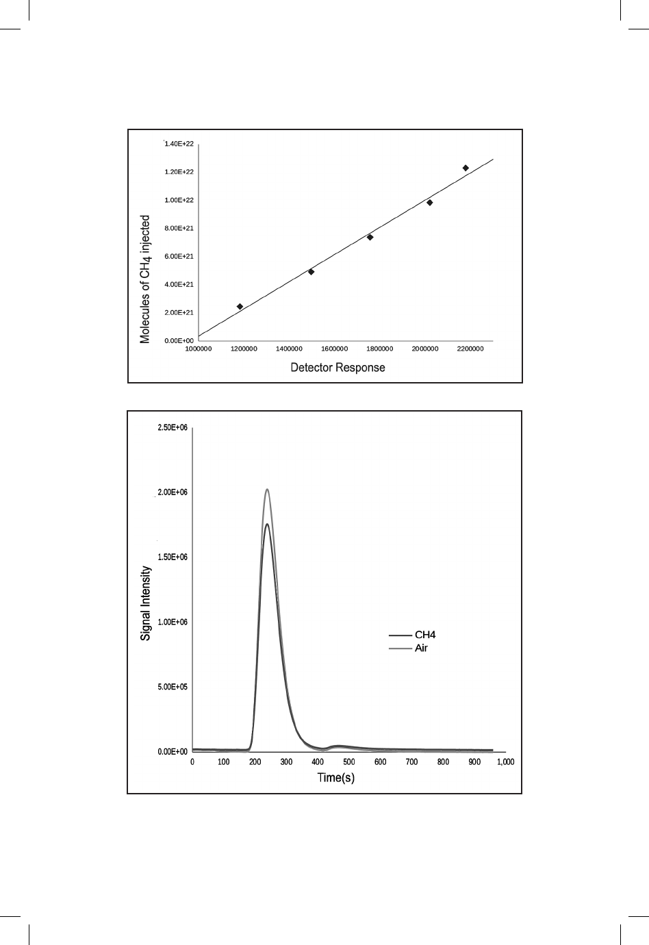
After injecting known volumes of gas, the equa-

tion PV=nRT and Avogadro’s number were used to calculate

the number of molecules per sample. The calibration curve

is shown in Figure 4 (below). The peaks on Figure 3. show

the retention time and concentration of molecules of meth-

ane. Because the volumes were known, we were able to use

the equation PV=nRT and determine the number of moles

in the sample. Then, using Avogadro’s number of 6.23x10

atoms per mol, the number of atoms per sample was cal-

culated. The number of moles were then compared to the

voltage. Using this information when sample gas was passed

through the TCD, the voltage was then used to calculate concen-

tration. Table 1. denes the variables of the ideal gas equation.

By plotting the response of the TCD to varying volumes

of methane, a line was established with a correlation (r

) value of

.9883. This correlation shows the fraction of the value that was

derived from the data, and what was derived from tting the trend

line. A value of 0.9883 shows that the line was derived at 98.83%

of data, and that there is only a 1.17% error due to tting the line.

Tests were run at a variety of temperatures, ranging from

30°C to 100°C, in order to ascertain where the best separation oc-

Determination of the Concentration of Atmospheric Gases

by Gas Chromatography

Table 1. Variables of the ideal gas equation.

P= Pressure = 1atm

V = Volume= volume of sample

N= number of moles= x

R= gas constant= .08206

T= temperature K°= 296.15 K°

Chris Haskin

Figure 4. Calibration Curve 1.

Figure 5. Room Air Compared to Methane using poraPLOT Column.

curs. Despite literature data showing otherwise

, it was decided

that the poraplot column was not separating the atoms of interest

(CH

). This is shown in Figure 5. By increasing the CH

concen-

tration, it was easier to map it, which led to the discovery that its

peak may have been lost in the nitrogen peak.

Figure 6. compares the room air to room air with added

methane. This graph shows that the room air sample (containing

nitrogen, oxygen and methane) is not resolved into three compo-

nent peaks. Because the methane peak begins so close to the end

of the nitrogen peak, and the methane is very dilute in room air

samples, it is very likely the two species are eluting at the same

time. Measures were taken to add to molecule retention time and

allow for a more distinct chromatogram, but at this time we have

Determination of the Concentration of Atmospheric Gases

by Gas Chromatography

Figure 6. Comparison between Room Air and Room Air+Methane

not perfected the method. Also note that in Figure 6. the chro-

matogram of room air shows that the nitrogen peak is cut off, be-

cause the TCD only records voltage up to 6x10

microvolts (6V).

To solve the problem of poor methane separation, a

packed molecular sieve column was added to the loop. The col-

umn used is a Restek Moleseive column with a 2 mm inside di-

ameter, packed with 5 angstrom diameter Zeolite packing. Tests

were run with the new column added in the loop, yet there were

still difculties in isolating the methane. The ow rate was low-

ered to nearly 2mL/ min in order to give the molecules more

time in the columns, and thus more time to adhere to the station-

ary phase. Problems with the separation continued, thus the next

step was to place the sample loop into an ice bath in order to cool

the sample molecules. By cooling the sample, the molecules

should in turn have slowed down, increasing chances of separa-

tion. There were still problems differentiating a proper methane

peak with room air samples. Our samples were then re-tested,

using only the molecular sieve column. Successful separation

of methane, oxygen and nitrogen was observed; the poraPLOT

column was removed and the experiments continued with the

molecular sieve column only.

Sample Analysis

Sample atmosphere bags were connected to a 6 port

valve system. This system has two settings: analyze mode and

fill mode. In fill mode, the gas pump sucks sample atmosphere

out of the bag and into the sample loop. The carrier gas must

always run through the column, so in both analyze and fill mode

the Hydrogen ows into the GC, and thus the column. Once the

sample loop is full, the system is put into analyze mode and the

valve switches so that the carrier gas pushes through the sample

loop and into the GC. This in turn pushes the sample atmosphere

into the GC and detector. After discovery of the poraPLOT not

separating methane molecules, the poraPLOT was replaced by

the mol sieve column. This provided better resolution and sepa-

ration than the poraPLOT column. A septum port was also added

to the sample loop for direct injections of atmosphere gas.

Chris Haskin

Data Analysis

Once the calibration curve was established and TCD re-

sponse was recorded, samples of room air were tested, as methane

concentrations in indoor air are similar to those found outside.

The room air samples delivered 2 peaks in chromatograms; the

rst was determined to be Oxygen (O

), and the second was deter-

mined to be Nitrogen (N

). The peaks were determined by intro-

ducing pure forms of the gases to the system in order to determine

where Oxygen and Nitrogen eluted. Figure 7. shows a sample

chromatogram of room air.

This chromatogram shows that the typical peaks of O

and

, but CH

seem to be below the limit of detection for this small

(1mL) sample size. The CH

retention time falls in the latter part

of the N

peak. In order to show the comparison of methane and

room air, methane was added to a bag of pure air from a cylinder.

In higher concentrations it is much easier to see where the peaks

should be, and to compare them to room air. Figure 8. shows a

comparison of room air and room air doped with methane from

the house tap.

Using the sample bag with added methane shows the peak

beginning as the large nitrogen peak is still attening out. The fol-

Determination of the Concentration of Atmospheric Gases

by Gas Chromatography

Figure 7. Sample Chromatogram of Room Air

Chris Haskin

Figure 8. Illustration of a Bag of Room Air and Room Air + Methane

Figure 9 Chromatogram using Molsieve column

lowing diagram, Figure 9., illustrates the air + methane reference

sample matched up to atmospheric air analyzed using only the

molecular sieve column. A discernible peak, although small, can

be viewed just to the right of the nitrogen peak. Figure 9. shows

the molsieve chromatogram.

DISCUSSION

While the research is ongoing a viable separation technique

for methane is within reach. As more adjustments are made the ma-

chine should prove quite useful for atmospheric measurements.

While previous data and the literature suggested that the

poraPLOT column was the correct column for analyzing CH

proper separation was never achieved with this column in place.

One possible reason for this is that without proper equipment, the

temperature of the sample could not be lowered enough. Cryo-

genic trapping is a technique used to narrow the width of sample

peaks and thus improve resolution in chromatograms. The tech-

nique involves lowering the temperature of analytes far below am-

bient temperature (as low as -180° C), then releasing them from

the trap by very rapid heating (60° C/ min). A version of this was

attempted using ice baths, but was found not to be effective.

Another way that poor separation was addressed was by

adding volume to the sample loop. It was thought that 1mL sam-

ples were not large enough to achieve proper separation. To x

this the sample, loop size was increased. Even with larger sample

sizes good separation did not occur.

This experiment was conducted in order to prepare an

instrument for further research. It has been shown that this is a

viable instrument in atmospheric chemistry. This project will con-

tinue, and in future writings data from other sources and locations

will be analyzed.

Determination of the Concentration of Atmospheric Gases

by Gas Chromatography

REFERENCES

Jacob, D. J.; Introduction to Atmospheric Chemistry. Princeton University Press: Princeton,

NJ,1999, 115

Butler, J.H.; The NOAA Annual Greenhouse Gas Index. http://www.esrl.noaa.gov/gmd/

aggi/ , 2012.

Harris, D.C. Exploring Chemical Analysis. W.H. Freeman and Company: New York, NY,

2009.

Oregon State University. Ice Cores Reveal Fluctuations in Earth’s Greenhouse Gases.

http://www.sciencedaily.com /releases/2008/05/080514131131.htm, 2013.

American Chemical Society. What are the greenhouse gas changes since the Industrial

Revolution?http://portal.acs.org/portal/acs/corg/content?_nfpb=true&_

pageLabel=PP_SUPERARTICLE&node_id=859&use_sec=false&sec_url_

var=region1&__uuid=501cfc97-a24a-492c-9efe-422171c9d620, 2013.

Intergovernmental Panel on Climate Change. What factors Determine Earth’s Climate.

http://www.ipcc.ch/publications_and_data/ar4/wg1/en/faq-1-1.html 2012 .

Wayne, R.P. Chemistry of Atmospheres, 2nd ed.; Clarendon Press: Oxford,1991.

Wood, R. &et al.; Shale Gas: aprovisional assessment of the climate change and

environmental impacts. AReport commissioned by the Cooperative and

undertaken by researchers at the Tyndall Centre, University of Manchester.

2011; Scinder (accessed March 2013).

Howarth,R.W., Santoro, R., Ingraffea, A.; Methane and greenhouse-gas footprint of natural

gas from shale formations. Climatic Change. June 201, vol. 106, issue 4, pp.

679-690 (accessed March 2013).

Thet, K., Woo, N.; Gas Chromatography. U. C. Davis Chem Wiki;

http://chemwiki.ucdavis.edu/Analytical_Chemistry/Instrumental_Analysis/Gas_

Chromatography 2013.

Harvey. D. Analytical Chemistry 2.0. [Online Text]; http://www.asdlib.org/onlineArticles/

ecourseware/Analytical%20Chemistry%202.0/Welcome.html 2013.

Merriam-Webster; Merriam-Webster.com; http://www.merriam-webster.com/dictionary/

permanent%20gases, (2013).

Vickers, A.K. Columns Used for the Analysis of Renery and Petrochemical Products by

Cappilary GC; Agilent Technologies. http://www.chem.agilent.com/Library/

posters/Public/Columns%20Used%20for%20the%20Analysis%20of%20

Renery%20and%20Petrochemical%20Products%20by%20Capillary%20GC.

pdf, 2013.

Chris Haskin