
2020
Perez, Marcie
Texas A&M Transportation Institute
6/8/2020
PivotTable Basics
1
According to Microsoft, a PivotTable “is an interactive way to quickly summarize large amounts of data”
(Microsoft, 2020). A PivotTable can also allow you to take a quick look at a data set and help you make
decisions on how you want to proceed. I use them in both manners. For researchers, I often use
PivotTables to summarize data for use in reports and infographics, but I also use PivotTables to make
decisions on how to proceed with a data set, and that has been invaluable.
The following are examples to help you learn to make basic PivotTables in Microsoft Excel. We will be
working with Fatal Analysis Reporting System (FARS) data related to Texas fatal crashes in 2018
(National Highway Traffic Safety Administration, 2020). To practice along with the presentation, you will
need:
• A computer with a recent version of Microsoft Excel
• A copy of the file 2018_FARS_CRASH_DATA
The Data
Open the excel file. The first sheet in the file contains the FARS data we will be using. It contains 3,305
records, and the data is displayed in 15 columns (A-O). FARS data comes in a coded format, but for this
tutorial the data has been decoded. The following are a list of the variable names in the data.
• RECORD
• STATE
• DAY
• MONTH
• YEAR
• DATE
• FATALS
• HOUR
• COUNTY NAME
• CITY NAME
• DAY OF WEEK
• FUNCTIONAL SYSTEM
• HARMFUL EVENT
• MANNER OF COLLISION
• LIGHT CONDITION
PivotTable Practice
The following instructions will help you build PivotTables in the other tabs in the file.
Crashes by County PivotTable
1. Click on the second tab named 2. CRASHES BY COUNTY. You should see a PivotTable with the
count and percentage of crash for each county in Texas and an area where to build a new

2
PivotTable.
2. Click in the box that says PivotTable4. On the right side of your screen, the PivotTable Fields
should open.
3. Now click on the PivotTable with the list of counties, the count of fatal crashes, and the
percentage of crashes by county. The PivotTable Fields boxes should now contain information.

3
For this exercise we will recreate the Crashes by County PivotTable in PivotTable4.
4. Click on the PivotTable4 box, in the sheet.
5. From the list of variables in the PivotTable Fields panel on the right, click on the County Name
variable and drag it to the box labeled Rows at the bottom left corner of the PivotTable Field
Box.
6. Click and drag the variable RECORD to the box labeled Values at the bottom right corner of the
PivotTable Fields Panel. Notice that the variable label changes to Sum of RECORD.
7. Click on the Sum of RECORD. You should see a list of options pop-up.
8. Click on Value Field Settings. A box with a list of mathematical options should pop-up and Sum
should be highlighted.
9. Click on Count from the calculation options,

4
10. At the top change the Custom Name field to say Crashes and then click OK. Now the PivotTable
should be showing the number of records by county.
11. Click and drag the RECORD variable to the Values box again.
12. Open the Value Field Settings and change Sum to Count, as you did before.
13. Click on the second tab, Show Values As, in the Value Field Settings Box.
14. From the Show Values As dropdown box select % of Column Total.
15. Change the Custom Name to Percent of Crashes and click OK.
16. Now that you have a crash count and the percent of crashes for each county, right click on a
percent in the column.

5
17. Select Sort for the pop-up and then Sort Largest to Smallest.
18. Click an empty cell in the spreadsheet. You should have two identical PivotTables.
Pivot Table Filters
1. Click on the third tab 3. DAY AND LIGHTING. You should see a PivotTable with the days of the
week in the first column, lighting conditions in the top row, and counts of the number of records

6
in each category.
2. Click inside the PivotTable so you can see the PivotTable Fields. You will now change the
PivotTable so that you only see one Lighting Condition at a time.
3. In the PivotTable Fields Panel, you will see the LIGHT CONDITION variable in the top right box
labeled Columns. Click on LIGHT CONDITION and drag it to the left to the Filters box. The
PivotTable should now show only one list of values, and you will see a dropdown box above the

7
table (shown in the red circle).
4. The Light Condition Filter, above the table, shows (All). Click on the dropdown arrow and select
Daylight and then click OK.
5. We see that Wednesday has the most number of fatal crashes. Now we want to change the
PivotTable to show the number of crashes by day for dark conditions.
6. When you click again on the Light Condition Dropdown arrow, you see three different dark
lighting conditions. Below the list of lighting conditions there is a Select Multiple Items check
box. Check the box.

8
7. Select the three different dark lighting conditions: Dark – Lighted, Dark - Not Lighted, and Dark -
Unknown Lighting. Uncheck the Daylight condition and click OK.
8. Now you can see that Sunday has the highest number of fatal crashes in dark conditions.

9
9. Now we can make a visualization of this data. Select the Insert Table from the top menu ribbon
bar.
10. Select the first 2D bar chart from the ribbon bar.

10
11. A chart illustrating the data should pop-up and if you change the filters on the chart or the
PivotTable the data will change.
Create a New PivotTable
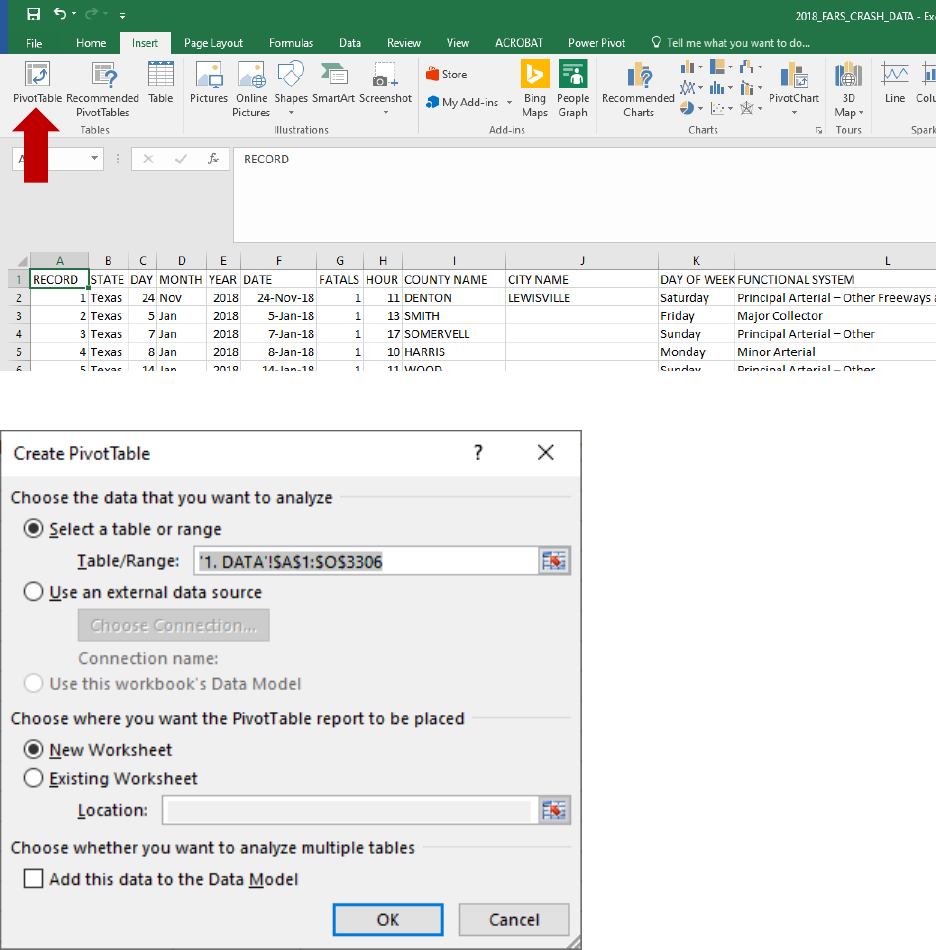
1. Click on the first tab 1. DATA.
2. Click in Cell 1A. It contains the word “RECORD”.
3. Click Insert on the top ribbon bar.
11
4. From the Insert Ribbon Bar select the icon for PivotTable.
5. You will see a pop-up window with the location of the data to be used in the PivotTable ('1.
DATA'!$A$1:$O$3306) and the location where the PivotTable will go (New Worksheet). Click OK.
6. A new worksheet will open with a PivotTable box. Now you can drag the variables into the
locations you want.
Things to Remember
• If you change your data be sure to Refresh the PivotTable.
• Check your calculations. Do you want count or sum the data?
• Check your percentages. Do you want the percent by column or row?
• If you share your PivotTables, be sure to add a detailed description of what the PivotTable
shows and always keep a copy of the original file.
12
References
Microsoft. (2020). Support. Retrieved from Microsoft: https://support.microsoft.com/en-
us/office/overview-of-pivottables-and-pivotcharts-527c8fa3-02c0-445a-a2db-
7794676bce96?ui=en-us&rs=en-us&ad=us
National Highway Traffic Safety Administration. (2020). Fatality Analysis Reporting System. Retrieved
from https://www.nhtsa.gov/crash-data-systems/fatality-analysis-reporting-system
