
Tutorial for VCS
STEP 1: login to the Linux system on Linuxlab server. Start a terminal (the
shell prompt).
Click here to open a shell window
Fig. 1 The screen when you login to the Linuxlab through equeue
STEP 2: In the terminal, execute the following command:
module add ese461
You could perform “module avail” in the terminal to find the available
modules on Linuxlab. Make sure ese461 is presented when you execute
this command.
1.Find the available modules
3.This command will set up the work
environment for class ESE461
2.Make sure ese461 is presented
Fig. 2 Build work environment for class ESE461 using module
1

STEP 3: Getting started with Verilog
• Creating a new folder (better if you have all the files for a project in a
specific folder).
• Enter into this new folder and start writing your Verilog script in a
new file (.v file). Example code for modeling an counter is here
• In addition to model code, Test Bench script has to be given in order
to verify the functionality of your model (.v file). Example code of test
bench for counter is here.
Use gedit to edit the .v files
(gedit is a commonly used GUI editor on Linux )
Fig. 3 Open gedit through teminal
STEP 4: Compiling and simulating your code
• In the terminal, change the directory to where your model and test
bench files (Counter.v and Counter_tb.v) are present by using this
command:
cd <path>
For example:
cd ~/ESE461/VcsTutorial/
(Remark: ‘~’ means home directory on Linux)
• Compile the files by typing in the terminal:
vcs <file>.v <file_tb>.v
In the above example, it should be:
vcs Counter.v Counter_tb.v
There should be no error presented in the terminal. Otherwise you
need to check your code and correct them according to the related
message. The complier will print out detailed information about your
mistakes in the code.
2

Successfully compiled
Fig. 4 The result of successfully executing vcs
Don’t need to recompile
because nothing changed
Fig. 5 The result of recompile the code when nothing changed
3

Error message when encounter a
error during the compiling process.
Fig.6 The result of vcs when it thinks there are mistakes in the code
• A successfully compiling will print out on terminal “../simv up to
date”. And it should generate an executable file named “simv” in the
same folder where your codes are present.
• Then in the terminal run:
./simv
• After the process finishes, “VCS Simulation Report” will be present
on the terminal and a file named “<file>.vcd” will be generated in the
same folder where your codes are present. This is the dump file we
specified in the test bench code and we will use it to graphically
display the simulation results.
Simulation Report
Fig. 7 Simulation Report
STEP 5: Displaying your Results graphically using dve
• After simulation report and “<file>.vcd” is generated, now type the
following command in the terminal:
dve
This is a viewer to plot and verify your results.
(Remark: an “&” can be placed behind the command, which means
this command will run in background, so the terminal will be
released)
4

Fig. 8 Start dve on the terminal
• Go to “File/Open Database” and select the “.vcd” file from the
project folder.
Fig. 9 dve open database (1)
Select the .vcd file
Fig. 10 dve open database (2)
5

• Then you will find the name of your test bench model in the
Hierarchy box (Counter_tb here). Expand it so that you can find DUT
in the options.
The module name of the test bench
Fig. 11 dve open database (3)
•
If you click on DUT , select the signals listed(all or partial) and right
click, you will find an option “Add to Waves”.
Device(Module)
under test
Select them and right
click the mouse
Fig. 12 dve open database (4)
6

• Click on “Add to New Wave View” to see the waveforms of your
Inputs and Outputs. You should see your results in a new window.
Then adjust the size of the waveform and explore other options as
well.
Adjust the size of waveform.
The leftmost is “fit the screen”
Fig. 13 The waveform display
7
Additional Option to run in Debug mode:
Instead of compiling the files directly as before, we can enable a debug flag
during compilation by using following command
vcs -lca -debug_access+all Counter.v Counter_tb.v
Now run the code:
./simv -gui &
This should open the dve tool automatically and you can fully run your test
bench or debug it step by step. To do this first select inputs and outputs
from variable window and right click “Add to the Waves” as before. This
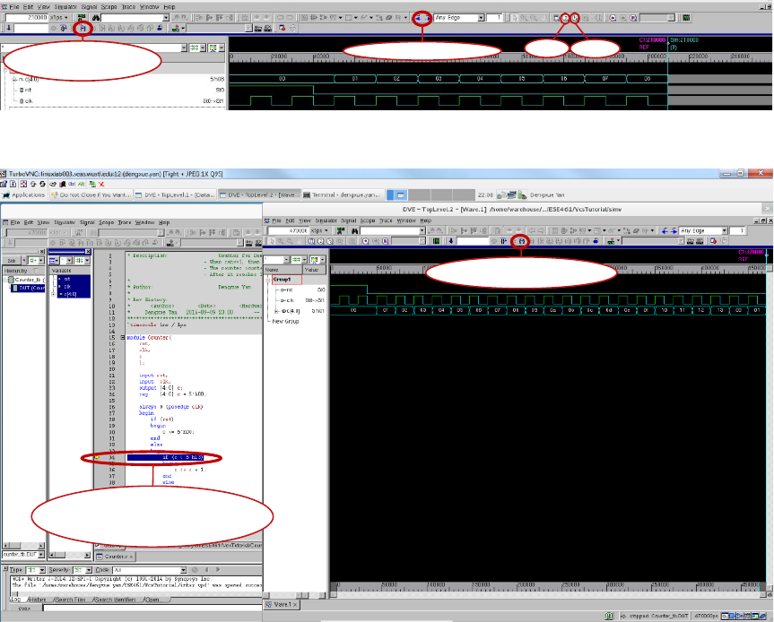
should open the following window as shown in the Fig. 14 . Then click the
tool button of blue arrow in brace or press F11 to run the test bench step
by step(Fig. 14 and Fig. 15). Or click the tool button of the blue arrow
pointing downward or press F5 to run the test bench fully(Fig. 16 ~ Fig. 18).
Other tool options are also available and just explore them by yourself.
Click here or press “F11” to
run the test bench step by step
move REF cursor front and back
Zoom In
Zoom Out
Fig. 14 The waveform display in debug mode
The cursor indicates which line of code the
simulator is executing when click “Step ” button
Click here or press “F11" to run the
test bench step by step
Fig.15 The code trace cursor in debug mode
8

2.The report indicates the simulation has finished
1.Click here or press
“F5” to run simulation
3.Fit screen
Fig.16 Fully “run” in debug mode(1)
4.Click here or press “F5"
again will reset the simulation
6.Fit screen
5.The report indicates the simulation has reset
Fig.17 Fully “run” in debug mode(2) – simulation reset
9

8.The report indicates the simulation has finished
7.Then click here or press “F5”
will restart the simulation
9.Fit screen
Fig.18 Fully run in debug mode(3) -- simulation restart
10

