The Effect of Home-Sharing on House Prices and Rents: Evidence from AirbnbWe thank Don Davis, Richard Green, Chun Kuang, Aske Egsgaard, Tom Chang, and seminar participants at the AREUA National Conference, the RSAI Annual Meetings, the Federal Reserve Bank of San Francisco, the UCI-UCLA-USC Urban Research Symposium, and the PSI Conference for helpful comments and suggestions. All errors are our own.

The Eﬀect of Home-Sharing on House Prices and Rents:

Evidence from Airbnb

∗

Kyle Barron

†

Edward Kung

‡

Davide Proserpio

Abstract

We assess the impact of home-sharing on residential house prices and rents. Using a dataset

of Airbnb listings from the entire United States and an instrumental variables estimation strat-

egy, we show that Airbnb has a positive impact on house prices and rents. This eﬀect is stronger

in zipcodes with a lower share of owner-occupiers, consistent with non-owner-occupiers being

more likely to reallocate their homes from the long- to the short-term rental market. At the

median owner-occupancy rate zipcode, we ﬁnd that a 1% increase in Airbnb listings leads to

a 0.018% increase in rents and a 0.026% increase in house prices. Finally, we formally test

whether the Airbnb eﬀect is due to the reallocation of the housing supply. Consistent with

this hypothesis, we ﬁnd that, while the total supply of housing is not aﬀected by the entry of

Airbnb, Airbnb listings increase the supply of short-term rental units and decrease the supply

of long-term rental units.

Keywords: Sharing economy, peer-to-peer markets, housing markets, Airbnb

∗

We thank Don Davis, Richard Green, Chun Kuang, Aske Egsgaard, Tom Chang, and seminar participants at

the AREUA National Conference, the RSAI Annual Meetings, the Federal Reserve Bank of San Francisco, the UCI-

UCLA-USC Urban Research Symposium, and the PSI Conference for helpful comments and suggestions. All errors

are our own.

†

NBER; [email protected].

‡

Department of Economics, UCLA; [email protected].

Marshall School of Business, USC; [email protected].

Electronic copy available at: https://ssrn.com/abstract=3006832

1 Introduction

The sharing economy represents a set of peer-to-peer online marketplaces that facilitate matching

between demanders and suppliers of various goods and services. The suppliers in these markets

are often small (mostly individuals), and they often share excess capacity that might otherwise go

unutilized—hence the term “sharing economy.” Economic theory would suggest that the sharing

economy improves economic eﬃciency by reducing frictions that cause capacity to go underutilized,

and the explosive growth of sharing platforms (such as Uber for ride-sharing and Airbnb for home-

sharing) testiﬁes to the underlying demand for such markets.

The growth of the sharing economy

has also come at the cost of great disruption to traditional markets (Zervas et al., 2017) as well

as new regulatory challenges, leading to contentious policy debates about how best to balance

individual participants’ rights to freely transact, the eﬃciency gains from sharing economies, the

disruption caused to traditional markets, and the role of the platforms themselves in the regulatory

process.

Home-sharing, in particular, has been the subject of intense criticism. Namely, critics argue

that home-sharing platforms like Airbnb raise the cost of living for local renters while mainly

beneﬁtting local landlords and non-resident tourists.

It is easy to see the economic argument. By

reducing frictions in the peer-to-peer market for short-term rentals, home-sharing platforms cause

some landlords to switch from supplying the market for long-term rentals—in which residents are

more likely to participate—to supplying the short-term market—in which non-residents are more

likely to participate. Because the total supply of housing is ﬁxed or inelastic in the short run, this

drives up the rental rate in the long-term market. Concern over home-sharing’s impact on housing

aﬀordability has garnered signiﬁcant attention from policymakers and has motivated many cities

to impose stricter regulations on home-sharing.

These frictions could include search frictions in matching demanders with suppliers and information frictions

associated with the quality of the good being transacted or with the trustworthiness of the buyer or seller. See Einav

et al. (2016) for an overview of the economics of peer-to-peer markets including the speciﬁc technological innovations

that have facilitated their growth.

Another criticism of Airbnb is that the company does not do enough to combat racial discrimination on its

platform (Edelman and Luca, 2014; Edelman et al., 2017) or that it generates negative externalities for neighbors

(Filippas and Horton, 2018) though we will not directly address these issues in this paper.

For example, Santa Monica outlaws short-term, non-owner-occupied rentals of fewer than 30 days as does New

York State for apartments in buildings with three or more residences. San Francisco passed a 60-day annual hard

cap on short-term rentals (which was subsequently vetoed by the mayor). It is unclear, however, to what degree to

which these regulations are enforced.

Electronic copy available at: https://ssrn.com/abstract=3006832

Whether or not home-sharing increases housing costs for local residents is an empirical question.

There are a few reasons why it might not. The market for short-term rentals may be very small

compared to the market for long-term rentals. In this case, even large changes to the short-term

market might not have a measurable eﬀect on the long-term market. The short-term market could

be small—even if the short-term rental rate is high relative to the long-term rate—if landlords prefer

more reliable long-term tenants and a more stable income stream. Alternatively, it is possible that

home-sharing simply does not cause much reallocation from the long-term rental stock to the short-

term rental stock. Owner-occupiers—those who own the home in which they live—may supply the

short-term rental market with spare rooms and cohabit with guests or they may supply their entire

home during temporary absences,

but either way, the participation of owner-occupiers in the short-

term rental market may not cause a reallocation from the long-term rental stock if these housing

units are still primarily used as long-term rentals in the sense that the owners are renting long-term

to themselves. Another type of participation in the short-term rental market that would not result

in reallocation is vacation homes that would not have been rented to long-term tenants anyway,

perhaps due to the restrictiveness of long-term leases causing vacation home-owners to not want to

rent to long-term tenants. In this case, the vacation home units were never part of the long-term

rental stock to begin with. In either case, whether owner-occupiers or vacation-home owners, these

homes would not be made available to long-term tenants independently of the existence of a home-

sharing platform. Instead, home-sharing provides these owners with an income stream for times

when their housing capacity would otherwise be underutilized.

In this paper, we study the eﬀect of home-sharing on residential house prices and rents using

a comprehensive dataset of all U.S. properties listed on Airbnb, the world’s largest home-sharing

platform. The data are collected from public-facing pages on the Airbnb website between 2012 and

the end of 2016, covering the entire United States. From this data, we construct a panel dataset of

Airbnb listings at the zipcode-year-month level. From Zillow, a website specializing in residential

real estate transactions, we obtain a panel of house price and rental rate indices, also at the zipcode-

year-month level. Zillow provides a platform for matching buyers and sellers in the housing market

and landlords with tenants in the long-term rental market; thus, their price measures reﬂect sale

A frequently cited example is that of the ﬂight attendant who rents out his or her home on Airbnb while traveling

for work.

Electronic copy available at: https://ssrn.com/abstract=3006832

prices and rental rates in the market for long-term housing. Finally, we supplement this data with

a rich set of time-varying zipcode characteristics collected from the Census Bureau’s American

Community Survey (ACS) and a set of variables correlated with tourism demand such as hotel

occupancy rates from STR, airport travelers from the Bureau of Transportation Statistics (BTS),

and hotels’ online reviews from TripAdvisor.

In the raw correlations, we ﬁnd that the number of Airbnb listings in zipcode i in year-month

t is positively associated with both house prices and rental rates. In a baseline OLS regression

with no controls, we ﬁnd that a 1% increase in Airbnb listings is associated with a 0.1% increase

in rental rates and a 0.18% increase in house prices. Of course, these estimates should not be

interpreted as causal and may instead be picking up spurious correlations. For example, cities that

are growing in population likely have rising rents, house prices, and numbers of Airbnb listings

at the same time. We therefore exploit the panel nature of our dataset to control for unobserved

zipcode level eﬀects and arbitrary city level time trends. We include zipcode ﬁxed eﬀects to absorb

any permanent diﬀerences between zipcodes while ﬁxed eﬀects at the Core Based Statistical Area

(CBSA)-year-month level control for any shocks to housing market conditions that are common

across zipcodes within a CBSA.

We further control for unobserved zipcode-speciﬁc, time-varying factors using an instrumental

variable that is plausibly exogenous to local zipcode level shocks to the housing market. To con-

struct the instrument, we exploit the fact that Airbnb is a young company that has experienced

explosive growth over the past ﬁve years. Figure 1 shows worldwide Google search interest in Airbnb

from 2008 to 2016. Demand fundamentals for short-term housing are unlikely to have changed so

drastically from 2008 to 2016 as to fully explain the spike in interest, so most of the growth in

Airbnb search interest is likely driven by information diﬀusion and technological improvements to

Airbnb’s platform as it matures as a company. Neither of these should be correlated with local zip-

code level unobserved shocks to the housing market. By itself, global search interest is not enough

for an instrument because we already control for arbitrary CBSA level time trends. We therefore

interact the Google search index for Airbnb with a measure of how “touristy” a zipcode is in a

base year, 2010. We deﬁne “touristy” to be a measure of a zipcode’s attractiveness for tourists and

The CBSA is a geographic unit deﬁned by the U.S. Oﬃce of Management and Budget that roughly corresponds

to an urban center and the counties that commute to it.

Electronic copy available at: https://ssrn.com/abstract=3006832

proxy for it using the number of establishments in the food service and accommodations industry.

These include eating and drinking places as well as hotels, bed and breakfasts, and other forms

of short-term lodging. The identifying assumptions of our speciﬁcation are that: 1) Landlords in

more touristy zipcodes are more likely to switch into the short-term rental market in response to

learning about Airbnb than landlords in less touristy zipcodes and 2) ex-ante levels of touristiness

are not systematically correlated with ex-post unobserved shocks to the housing market at the

zipcode level that are also correlated in time with Google search interest for Airbnb. We discuss

the instrument, its construction, and exercises supporting the exclusion restriction in more detail

in Sections 5, 5.1, and in the Appendix B.

Using this instrumental variable, we estimate that for zipcodes with the median owner-occupancy

rate (72%), a 1% increase in Airbnb listings leads to a 0.018% increase in the rental rate and a

0.026% increase in house prices. We also ﬁnd that the eﬀect of Airbnb listings on rental rates and

house prices is decreasing in the owner-occupancy rate. For zipcodes with a 56% owner-occupancy

rate (the 25th percentile), the eﬀect of a 1% increase in Airbnb listings is 0.024% for rents and

0.037% for house prices. For zipcodes with an 82% owner-occupancy rate (the 75th percentile),

the eﬀect of a 1% increase in Airbnb listings is only 0.014% for rents and 0.019% for house prices.

These results are robust to a number of sensitivity and robustness checks that we discuss in detail

in Sections 5.1 and 6.2.

The fact that the eﬀect of Airbnb is moderated by the owner-occupancy rate suggests that the

eﬀect of Airbnb could be driven by non-owner occupiers being more likely (because of Airbnb) to

reallocate their housing units from the long- to the short-term rental market. We directly test this

hypothesis using the same instrumental strategy described above and data on various measures of

housing supply that we collected from the American Community Survey. We ﬁnd that: (i) the total

housing stock (which is the sum of all renter-occupied, owner-occupied, and vacant units) is not

aﬀected by the entry of Airbnb, (ii) an increase in Airbnb listings leads to an increase in the number

of units held vacant for recreational or seasonal use,

(iii) an increase in Airbnb listings leads to a

decrease in the number of units available to long-term renters, and (iv) the above eﬀects on supply

We focus on tourism because Airbnb has historically been frequented more by tourists than business travelers.

Airbnb has said that 90% of its customers are vacationers but is attempting to gain market share in the business

travel sector.

According to Census methodology, units without a usual tenant but rented occassionally to Airbnb guests would

be classiﬁed as vacant for recreational or seasonal use. We describe the data in more detail in Section 6.4.

Electronic copy available at: https://ssrn.com/abstract=3006832

are smaller for zipcodes with a higher owner-occupancy rate. These results are consistent with

the hypothesis that Airbnb increases rents and house prices by causing a reallocation of housing

supply from the long-term rental market to the short-term rental market. Moreover, the size of

the reallocation is greater in zipcodes with fewer owner-occupiers because, intuitively, non-owner-

occupiers may be more likely to reallocate. Finally, it is worth mentioning that we cannot rule out

the possibility of other eﬀects of Airbnb such as any of the positive or negative externalities; thus,

our results should be interpreted as the estimated net eﬀect with evidence for the presence of a

reallocation channel.

2 Related literature

We are aware of only two other academic papers that directly study the eﬀect of home-sharing on

housing costs, and both of them focus on a speciﬁc U.S. market. Lee (2016) provides a descriptive

analysis of Airbnb in the Los Angeles housing market while Horn and Merante (2017) use Airbnb

listings data from Boston in 2015 and 2016 to study the eﬀect of Airbnb on rental rates. Using

a ﬁxed eﬀect model, they ﬁnd that a one standard deviation increase in Airbnb listings at the

census tract level leads to a 0.4% increase in asking rents. In our data, we ﬁnd that a one standard

deviation increase in listings at the within-CBSA zipcode level in 2015-2016 implies a 0.54% increase

in rents.

We contribute—and diﬀerentiate from previous work—to the literature concerning the eﬀect

of home-sharing on housing costs in several important ways. First, we present the ﬁrst estimates

of the eﬀect of home-sharing on house prices and rents that use comprehensive data from across

the United States. Second, we are able to exploit the panel structure of our dataset to control

for unobserved neighborhood heterogeneity as well as arbitrary city-level time trends. Moreover,

we identify a plausible instrument for Airbnb supply and conduct several exercises to support its

validity. These exercises reassure us that the measured association between Airbnb and house prices

and rents is likely causal. Third, we show that the eﬀect of Airbnb is strongly moderated by the

rate of owner-occupiers, a ﬁnding consistent with the hypothesis that the Airbnb eﬀect operates

through the reallocation of housing supply from the long- to the short-term rental market. Fourth,

we provide direct evidence in support of this hypothesis by showing that Airbnb is associated with

Electronic copy available at: https://ssrn.com/abstract=3006832

a decrease in long-term rentals supply and an increase in short-term rentals supply while having no

association with changes in the total housing supply. Fifth, by showing that the eﬀects of Airbnb

are moderated by the owner-occupancy rate, our results highlight the importance of the marginal

homeowner in terms of reallocation (since owner-occupiers are much less likely to reallocate their

housing to the permanent short-term rental stock). Thus, the marginal propensity of homeowners

to reallocate housing from the long- to the short-term rental market is a key elasticity determining

the overall eﬀect of home-sharing.

Our paper also contributes to the growing literature on peer-to-peer markets. Such literature

covers a wide array of topics, from the eﬀect of the sharing economy on labor market outcomes

(Chen et al., 2017; Hall and Krueger, 2017; Angrist et al., 2017), to entry and competition (Gong et

al., 2017; Horton and Zeckhauser, 2016; Li and Srinivasan, 2019; Zervas et al., 2017), to trust and

reputation (Fradkin et al., 2017; Proserpio et al., 2017; Zervas et al., 2015). Because the literature

on the topic is quite vast, here we focus only on papers that are closely related to ours and refer

the reader to Einav et al. (2016) for an overview of the economics of peer-to-peer markets and to

Proserpio and Tellis (2017) for a complete review of the literature on the sharing economy.

Closely related to the marketing literature and this work we ﬁnd papers that study the eﬀects

of the entry of peer-to-peer markets and the competition that they generate. Gong et al. (2017),

for example, provide evidence that the entry of Uber in China increased the demand for new cars;

Farronato and Fradkin (2018), Li and Srinivasan (2019), and Zervas et al. (2017) study the eﬀect

of Airbnb on the hotel industry; however, each one of them focuses on a diﬀerent question. Zervas

et al. (2017) focus on the subsitution patterns between Airbnb and hotels, and show that, after

Airbnb entry in Texas, hotel revenue dropped. Moreover, the authors show that this negative

eﬀect is stronger in periods of peak demand. Farronato and Fradkin (2018) focus instead on the

gains in consumer welfare generated by the entry of Airbnb in 50 U.S. markets. Finally, Li and

Srinivasan (2019) study how the ﬂexible nature of Airbnb listings aﬀects hotel demand in diﬀerent

markets. The authors show that, in response to the entry of Airbnb, some hotels may beneﬁt

from moving away from seasonal pricing. Our paper looks at a somewhat unique context in this

literature because we focus on the eﬀect of the sharing economy on the reallocation of goods from

one purpose to another, which may cause local externalities. Local externalities are present here

because the suppliers are local and the demanders are non-local; transactions in the home-sharing

Electronic copy available at: https://ssrn.com/abstract=3006832

market, therefore, involve a reallocation of resources from locals to non-locals.

Our contribution

is therefore to study this unique type of sharing economy in which public policy may be especially

salient.

Finally, our work is related to papers studying the consequences of what happens when a online

platform lowers the cost to entry for suppliers. For example, both Kroft and Pope (2014) and

Seamans and Zhu (2013) study the impact of Craiglist on the newspaper industry and ﬁnd a

substantial substitution eﬀect between the two.

The rest of the paper is organized as follows. In Section 3, we discuss the economics of home-

sharing and how home-sharing might be expected to aﬀect housing markets. In Section 4, we

describe the data we collected from Airbnb and present some basic statistics. In Section 5, we

describe our methodology and present exercises in support of the exclusion restriction of our in-

strument In Section 6, we discuss the results and present several robustness checks to reinforce the

validity of our results. Section 7 discusses our ﬁndings, the limitations of our work, and provides

concluding remarks.

3 Theory

The market for long and short-term rentals is traditionally viewed as segmented on both the

supply and demand side. On the demand side, the demanders for short-term rentals are tourists,

visitors, and business travelers while the demanders for long-term rentals are local residents. On

the supply side, the suppliers of short-term rentals are traditionally hotels and bed and breakfasts

while the suppliers of long-term rentals are local landlords. Local residents who own their own

homes (owner-occupiers) are on both the demand and the supply side for long-term rentals (they

rent to themselves.)

Segmentation exists between the long- and short-term markets despite the fundamental simi-

larity in the product being oﬀered (i.e., space and shelter). The segmentation may exist for a few

reasons. First, short-term demanders may have very diﬀerent needs than long-term demanders.

Short-term demanders may only require a bed and a bathroom while long-term demanders may

This may not be seen as a real economic cost, though a shift of welfare from locals to non-locals is important

for public policy because policy is set locally. Some have also argued that home-sharing can create a real negative

spillover for neighbors (Filippas and Horton, 2018).

Electronic copy available at: https://ssrn.com/abstract=3006832

also require a kitchen and a living area. Second, the legal environment is very diﬀerent for short

and long-term demanders. Long-term tenants are typically aﬀorded rights and protections that are

not available to short-term visitors. Because of this segmentation, the unit price of renting exhibits

a term structure with the price of a short-term rental typically being much higher than the price

of a long-term rental. Marketplaces for long- and short-term rentals have historically remained

separate due to this segmentation.

Eﬀects of home-sharing: Housing supply reallocation and expansion

With the advent of home-sharing, segmentation on the supply side is becoming blurred. Because

of home-sharing platforms like Airbnb, it is now much easier for properties that were traditionally

used only for long-term rental to now also be used for short-term rental.

Now that it has become easier for owners of traditionally long-term housing to supply the

short-term market, what can we expect the eﬀects to be? First, we can expect some owners of

traditionally long-term housing to switch from supplying a long-term demander to supplying short-

term demanders. In the short run, the supply of housing and of hotels is inelastic, so this reduces

the supply of housing available in the long-term rental market and increases the supply of rooms

in the short-term rental market. This, in turn, pushes up rents in the long-term rental market

and pushes down rents in the short-term rental market (Horn and Merante, 2017; Zervas et al.,

2017). To the extent that search and matching frictions exist in both rental markets, this should

also reduce the vacancy rate in the long-term rental market and increase the vacancy rate in the

short-term rental market.

In the long run, we may also expect a supply response. The quantity of homes that are able

to supply both long- and short-term renters (i.e., homes traditionally built for long-term housing)

would be expected to increase in the long-run, while the quantity of hotel rooms that are only

able to supply the short-term market should decrease. The degree to which there will be quantity

adjustments will depend on the amount of land available in the city and the stringency of land use

regulations as well as the cost of construction (Gyourko and Molloy, 2015).

The size of the price and quantity response to home-sharing will also depend on the degree to

Home-sharing platforms greatly reduce traditional frictions that previously prevented some homeowners from

participating in the short-term rental market such as transactional frictions associated with trust (Einav et al., 2016).

Electronic copy available at: https://ssrn.com/abstract=3006832

which owners of traditionally long-term rental housing reallocate to the short-term rental market.

There are many reasons why an owner would choose not to reallocate. First and foremost, the

owner may live in her home. Thus, the owner will not reallocate from the long-term market (where

she rents to herself) to the short-term market. She may still participate in the short-term market by

selling unused capacity such as spare rooms or time when she is away, but this does not constitute

a reallocation from the long-term rental stock to the short-term rental stock because those spare

units of capacity would not have been allocated to a long-term tenant anyway and therefore does

not push up long-term rental rates. However, the allocation of spare capacity to the short-term

rental market, which constitutes a pure supply expansion, can reduce prices in the short-term rental

market.

Second, the owner may not reallocate from the long-term market to the short-term market

because the costs outweigh the beneﬁts. There could be many costs associated with supplying the

short-term rental market. Short-term renters may annoy neighbors, thus reﬂecting poorly on the

host and reducing his social capital in the community. In some cases, an owner may be bound

against renting to short-term renter by a homeowners’ association. Short-term renters may also

be more likely than long-term renters to cause property depreciation. A property owner may also

prefer the steadier stream of payments oﬀered by a long-term tenant over the lumpier stream of

payments oﬀered by sporadic visitors booking the home for short stays. Owners who simply choose

not to use the short-term market will cause no reallocation and therefore have no eﬀect on prices

in either the long-term or the short-term rental markets.

Finally, it is worth pointing out that reallocation from the long-term rental stock to the short-

term rental stock does not require that expected rents in the short-term rental market be higher

than expected rents in the long-term rental market. There may be reasons for preferring to rent

short-term instead of long-term even if the expected rents from short-term are lower, as may be

the case according to Coles et al. (2017). One reason could be that the owner does not like the

restrictiveness of a long-term lease. Even if the owner does not plan to use the property as a

primary residence or a vacation home, not renting to a long-term tenant increases the option value

for other uses such as letting family or friends stay or even holding out for higher long-term rents

If the owner-occupier is currently allocating spare rooms to the long-term market (i.e., by having a roommate)

and then decides to stop renting to a roommate and instead use Airbnb, then this would constitute a reallocation.

Electronic copy available at: https://ssrn.com/abstract=3006832

in the future while capitalizing on surges in short-term demand.

Eﬀects of home-sharing: Externalities and option value

Besides reallocation of housing supply, home-sharing can aﬀect long-term rental rates in a few other

ways. First, there may be both positive and negative externalities. On the positive side, home-

sharing may draw tourist money into the neighborhood, increasing revenues to local businesses and

increasing the demand for space in the neighborhoods. This would have the eﬀect of increasing both

long and short-term rental rates. Farronato and Fradkin (2018) and Coles et al. (2017) document

that home-sharing has drawn tourists into neighborhood that previously had very few, and Alyakoob

and Rahman (2018) ﬁnd a positive relation between Airbnb and restaurant employment. On the

negative side, the tourists that home-sharing draws in may be unpleasant or noisy. This can make

the neighborhood a more unpleasant place to live, thus decreasing rents. In local debates over

Airbnb, this has proven to be an unexpectedly salient point (Filippas and Horton, 2018).

Second, if tenants themselves are able to sell unused capacity in the short-term market, even

while under a long-term rental lease, then this would increase the demand for renting. In the short

run where supply is inelastic, this would push up rents in the long-term rental market. The degree

to which rents are increased depends on the degree to which tenants are willing and able to sell

unused capacity.

In the long-run, this eﬀect could lead to further expansion in housing supply.

So far, the discussion has focused on rental rates. Since buying a house can be viewed as

purchasing the present value of future rental payments, house prices should be equal to the ex-

pected present value of rents for a similar unit, adjusted for any tax implications, borrowing costs,

maintenance costs, and physical depreciation (Poterba, 1984). Thus, any eﬀect of home-sharing

on long-term rental rates will be directly capitalized into house prices. However, because home-

sharing also allows the homeowner to sell unused capacity on the short-term market, it should have

an additional eﬀect of increasing prices even further than the direct eﬀect on rents.

Finally, we note that it is possible that home-sharing externalities diﬀerentially aﬀect homeown-

ers and renters. For example, homeowners may be more sensitive to noisy neighbors than renters. If

such were the case, then the net eﬀect of home-sharing on the price-to-rent ratio could be negative

In practice, this will depend on the laws of individual cities and the types of leases landlords sign with tenants,

and the enforceability of any associated clauses.

Electronic copy available at: https://ssrn.com/abstract=3006832

even though the increased option value of using spare capacity would increase it.

Eﬀects of home-sharing: Other eﬀects

Finally, we note two other eﬀects that home-sharing may have on short and long-term rental

markets. First, in the long-run, home-sharing may change the characteristics of the housing stock.

For example, by increasing the option value of spare capacity, home-sharing may cause future homes

to be built with spare capacity in mind. There may be an increase in the supply of homes with

accessory dwelling units that are optimized for delivery to short-run tenants with the main unit

simultaneously being occupied by the owner.

Second, home-sharing may change the short-run supply elasticity of short-term rentals. Without

home-sharing, the short-run supply of short-term rentals is inelastic because there is only a ﬁxed

number of hotel rooms in any given neighborhood. High development costs and regulations make

it diﬃcult to adjust this number quickly. Home-sharing increases the ﬂexibility of traditionally

long-term housing to freely move between the long and short-term rental markets, thus leading to a

more elastic supply in the short-term market that is able to quickly expand in response to surges in

demand and then quickly contract when the surge is over. Farronato and Fradkin (2018) document

this phenomenon and evaluate its welfare implications.

Summary

To summarize, we have argued that home-sharing will have the following eﬀects. First, it will cause

a reallocation from the long-term housing supply to the short-term rental market. In the short-run,

this will push up rental rates and house prices, and decrease vacancy rates in the long-term market.

In the long-run, this could lead to an increase in housing supply, depending on the housing supply

curve of the market. Second, the size of the reallocation eﬀect will depend on the propensity of

homeowners to reallocate housing from the long-term market to the short-term market in response

to home-sharing. The eﬀect of home-sharing will be smaller when there are fewer homeowners

choosing to reallocate. Third, rents and prices should both increase due to the increased option

value of spare housing capacity, with prices increasing more than rents, thus leading to an increased

price-to-rent ratio. Countervailing these three eﬀects (which are all positive on prices and rents)

is the possibility of negative externalities. If home-sharing makes the neighborhood less desirable

Electronic copy available at: https://ssrn.com/abstract=3006832

to live in, then this could have a negative eﬀect on rents and prices. If homeowners are especially

sensitive to these externalities, home-sharing could decrease the price-to-rent ratio. On the other

hand, there could also be positive externalities that have the opposite eﬀects.

The predicted eﬀects of home-sharing on rental rates and house prices is therefore ambiguous.

In this paper, we aim simply to test for the net eﬀect. We will ﬁnd that the net eﬀect is positive

on rental rates, house prices, and the price-to-rent ratio in a way that is consistent with both the

reallocation channel and with increasing the option value of spare capacity. We also provide some

direct evidence of the reallocation channel. However, we cannot rule out the potential for other

eﬀects like externalities, nor do we disentangle the size of the various channels. It is also worth

mentioning that, in this paper, we focus only on short-run eﬀects. This choice is dictated by two

reasons: First, home-sharing is a relatively new phenomenon, and Airbnb itself is only a decade

old. Cities are still actively grappling with how to respond to home-sharing, and so we believe

that it is too early to look for long-run eﬀects. Second, in this paper, we do not ﬁnd any empirical

evidence that Airbnb (as yet) is associated with changes to the total housing supply, though we do

ﬁnd evidence for reallocation of housing from long-term rental stock to short-term rental stock.

4 Data and Background on Airbnb

4.1 Background on Airbnb

Recognized by most as the pioneer of the sharing economy, Airbnb is a peer-to-peer marketplace for

short-term rentals, where the suppliers (hosts) oﬀer diﬀerent kinds of accommodations (i.e. shared

rooms, entire homes, or even yurts and treehouses) to prospective renters (guests). Airbnb was

founded in 2008 and has experienced dramatic growth, going from just a few hundred hosts in 2008

to over three million properties supplied by over one million hosts in 150,000 cities and 52 countries

in 2017. Over 130 million guests have used Airbnb, and with a market valuation of over $31B,

Airbnb is one of the world’s largest accommodation brands.

4.2 Airbnb listings data

Our main source of data comes directly from the Airbnb website. We collected consumer-facing

information about the complete set of Airbnb properties located in the United States and about

Electronic copy available at: https://ssrn.com/abstract=3006832

the hosts who oﬀer them. The data collection process spanned a period of approximately ﬁve years,

from mid-2012 to the end of 2016. We performed scrapes at irregular intervals between 2012 to

2014 and at a weekly interval starting January 2015.

Our scraping algorithm collected all listing information available to users of the website, in-

cluding the property location, the daily price, the average star rating, a list of photos, the guest

capacity, the number of bedrooms and bathrooms, a list of amenities such as WiFi and air condi-

tioning, etc., and the list of all reviews from guests who have stayed at the property.

Airbnb host

information includes the host name and photograph, a brief proﬁle description, and the year-month

in which the user registered as a host on Airbnb.

Our ﬁnal dataset contains detailed information about 1,097,697 listings and 682,803 hosts span-

ning a period of nine years, from 2008 to 2016. Because of Airbnb’s dominance in the home-sharing

market, we believe that this data represents the most comprehensive picture of home-sharing in

the U.S. ever constructed for independent research.

4.3 Calculating the number of Airbnb listings, 2008-2016

Once we have collected the data, the next step is to deﬁne a measure of Airbnb supply. This task

requires two choices: First, we need to choose the geographic granularity of our measure; second,

we need to deﬁne the entry and exit dates of each listing in the Airbnb platform. Regarding

the geographic aggregation, we conduct our main analysis at the zipcode level for a few reasons.

First, it is the lowest level of geography for which we can reliably assign listings without error

(other than user input error).

Second, neighborhoods are a natural unit of analysis for housing

markets because there is signiﬁcant heterogeneity in housing markets across neighborhoods within

cities but comparatively less heterogeneity within neighborhoods. Zipcodes will be our proxy for

neighborhoods. Third, conducting the analysis at the zipcode level as opposed to the city level helps

with identiﬁcation. This is due to our ability to compare zipcodes within cities, thus controlling for

any unobserved city level factors that may be unrelated to Airbnb but that aﬀect all neighborhoods

In their paper, Horn and Merante (2017) incorrectly state that our Airbnb dataset comes form InsideAirbnb.com

(probably referencing an older version of this paper), but, in fact, the current results are based on data that one of

the authors of this paper scraped and collected.

Airbnb does not reveal the exact street address or coordinates of the property for privacy reasons; however, the

listing’s city, street, and zipcode correspond to the property’s real location.

Airbnb does report the latitude and longitude of each property but only up to a perturbation of a few hundred

meters. So it would be possible, but complicated, to aggregate the listings to ﬁner geographies with some error.

Electronic copy available at: https://ssrn.com/abstract=3006832

within a city such as a city-wide shock to labor productivity.

The second choice, how to determine the entry and exit date of each listing, comes less naturally.

First, our scraping algorithm did not constantly monitor a listing’s status to determine whether it

was active or not but rather obtained snapshots of the properties available for rent in the US at

diﬀerent points in time until the end of 2014 and at the weekly level starting in 2015. Second, even

if it did so, measuring active supply would still be challenging.

Thus, to construct the number of

listings going back in time, we employ a variety of methods following Zervas et al. (2017), which

we summarize in Table 1.

Table 1: Methods for Computing the Number of Listings

Listing is considered active ...

Method 1 starting from host join date

Method 2 for 3 months after host join date and after every guest review

Method 3 for 6 months after host join date and after every guest review

Method 1 is our preferred choice to measure Airbnb supply and will be our main independent

variable in all the analyses presented in this paper. This measure computes a listing’s entry date

as the date its host registered on Airbnb and assumes that listings never exit. The advantage of

using the host join date as the entry date is that for a majority of listings, this is the most accurate

measure of when the listing was ﬁrst posted. The disadvantage of this measure is that it is likely

to overestimate the listings that are available on Airbnb (and accepting reservations) at any point

in time. However, as discussed in Zervas et al. (2017), such overestimation would cause biases only

if, after controlling for several zipcode characteristics, it is correlated with the error term.

Aware of the fact that method 1 is an imperfect measure of Airbnb supply, we also experiment

with alternative deﬁnitions of Airbnb listings’ entry and exit. Methods 2 and 3 exploit our knowl-

edge of each listing’s review dates to determine whether a listing is active. The heuristic we use

is as follows: A listing enters the market when the host registers with Airbnb and stays active for

Estimating the number of active listings is a challenge even for Airbnb. Despite the fact that Airbnb oﬀers an

easy way to unlist properties, many times hosts neglect to do so, creating “stale vacancies” that seem available for

rent but in actuality are not. Fradkin (2015), using proprietary data from Airbnb, estimates that between 21% and

32% of guest requests are rejected due to this eﬀect.

The absence of bias in this measure is also conﬁrmed by Farronato and Fradkin (2018) where using Airbnb

proprietary data resulted in the same estimates obtained by Zervas et al. (2017) (where the data collection and

measures of Airbnb supply are similar to those used in this paper).

Electronic copy available at: https://ssrn.com/abstract=3006832

m months. We refer to m as the listing’s Time To Live (TTL). Each time a listing is reviewed,

the TTL is extended by m months from the review date. If a listing exceeds the TTL without any

reviews, it is considered inactive. A listing becomes active again if it receives a new review. In our

analysis, we test two diﬀerent TTLs, 3 months and 6 months.

Despite the fact that our diﬀerent measures of Airbnb supply rely on diﬀerent heuristics and

data, because of Airbnb’s tremendous growth, all our measures of Airbnb supply are extremely

correlated. The correlation between method 1 and each other measure is above 0.95 in all cases. In

the Appendix, we present robustness checks of our main results to the diﬀerent measures of Airbnb

supply discussed above and show that results are qualitatively and quantitatively unchanged.

4.4 Zillow: rental rates and house prices

Zillow.com is an online real estate company that provides estimates of house and rental prices

for over 110 million homes across the U.S. In addition to giving value estimates of homes, Zillow

provides a set of indexes that track and predict home values and rental prices at a monthly level

and at diﬀerent geographical granularities.

For house prices, we use the Zillow Home Value Index (ZHVI) that estimates the median

transaction price for the actual stock of homes in a given geographic unit and point in time. The

advantage of using the ZHVI is that it is available at the zipcode-month level for over 13,000

zipcodes.

For rental rates, we use the Zillow Rent Index (ZRI). Like the ZHVI, Zillow’s rent index is meant

to reﬂect the median monthly rental rate for the actual stock of homes in a geographic unit and

point in time. Crucially, Zillow’s rent index is based on rental list prices and is therefore a measure

of prevailing rents for new tenants. This is the relevant comparison for a homeowner deciding

whether to place her unit on the short-term or long-term market. Moreover, because Zillow is not

considered a platform for ﬁnding short-term housing, the ZRI should be reﬂective of rental prices in

the long-term market.

For each zipcode, we calculate the price-to-rent ratio as simply the ZHVI

One additional source of error in our computations is listings that were posted and then taken down between

2008 and 2011 since we did not start scraping until 2012. However, the number of such listings is likely to be small,

as shown in Figure 3. Moreover, our regressions use only data starting in 2011, so the inﬂuence on our results is likely

minimal. Further, as we show in Table 15 of the Appendix, our results are robust to the exclusion of early years.

Since the ZHVI and ZRI measure medians, our results only apply to the middle of the housing market. In the

Appendix, we explore eﬀects on diﬀerent segments of the housing market and ﬁnd that the eﬀects are qualitatively

similar.

Electronic copy available at: https://ssrn.com/abstract=3006832

divided by the ZRI.

4.5 Other data sources

We supplement the above data with several additional sources.

Variables used for the instrument We use monthly Google Trends data for the search term

“airbnb”, which we downloaded directly from Google. This index measures how often people

worldwide search for the term “airbnb” on Google and is normalized to have a value of 100 at

the peak month. We use the Census’s Zipcode Business Patterns data to measure the number of

establishments in the food services and accommodations industry (NAICS code 72) for each zipcode

in 2010.

Zipcode level time-varying characteristics We collect from the American Community Survey

(ACS) zipcode level annual estimates of median household income, population, share of 25-60 years

old with bachelors’ degrees or higher, and employment rate. From the ACS, we also obtain zipcode

level annual estimates of the number of housing units occupied by their owners or renters, and the

number of vacant units. The ACS also reports the reason a housing unit is vacant (for example,

whether the owner is holding it vacant so that he or she can use it occassionally for recreation or

whether it is vacant and currently looking for a tenant). We can therefore calculate the owner-

occupancy rate as the share of occupied units that are occupied by owners and the total housing

stock as the sum of owner-occupied units, renter-occupied units, and vacant units.

Proxies for tourism demand We obtained hotel occupancy rates at the CBSA-year-month

level from STR, a company that tracks hotel performance worldwide. We collected the number of

incoming airport travelers for all airports in the United States from the Bureau of Transportation

Statistics. Finally, we collected the complete set of hotel and restaurant reviews for all the hotels

and restaurants available on TripAdvisor. This data amount to about 18 million hotel reviews from

88,000 accommodation properties (hotels, inns, B&Bs) and about 25 million restaurant reviews

from about 478,000 restaurants from 2001 to the beginning of 2017 (2019 for restaurant reviews).

Electronic copy available at: https://ssrn.com/abstract=3006832

4.6 Summary statistics

Figure 2 shows the geographic distribution of Airbnb listings in June 2011 and June 2016. The map

shows signiﬁcant geographic heterogeneity in Airbnb listings with most Airbnb listings occurring in

large cities and along the coasts. Moreover, there exists signiﬁcant geographic heterogeneity in the

growth of Airbnb over time. From 2011 to 2016, the number of Airbnb listings in some zipcodes

grew by a factor of 30 or more; in others, there was no growth at all. Figure 3 shows the total

number of Airbnb listings over time in our dataset using methods 1-3. Using method 1 as our

preferred method, we observe that from 2011 to 2016, the total number of Airbnb listings grew by

a factor of 30, reaching over 1 million listings in 2016.

Table 2 gives a sense of the size of Airbnb relative to the housing stock at the zipcode level, for

the 100 largest CBSAs by population in our data. Even in 2016, Airbnb remains a small percentage

of the total housing stock for most zipcodes. The median ratio of Airbnb listings to housing stock

is 0.21%, and the 90th percentile is 1.88%. When comparing to the stock of vacant homes, Airbnb

begins to appear more signiﬁcant. The median ratio of Airbnb listings to vacant homes (either

for long- or short-term rental) is 2.63%, and the 90th percentile is 20%. Perhaps the most salient

comparison—at least from the perspective of a potential renter—is the number of Airbnb listings

relative to the stock of homes listed as vacant and for rent (which are part of the long-term rental

supply). This statistic reaches 13.7% in the median zipcode in 2016 and 129% in the 90th percentile

zipcode. This implies that in the median zipcode, a local resident looking for a long-term rental

unit will ﬁnd that about 1 in 8 of the potentially available homes are being placed on Airbnb instead

of being made available to long-term residents. Framed in this way, concerns about the eﬀect of

Airbnb on the housing market do not appear unfounded.

5 Methodology

Let Y

ict

be either the price index or the rent index for zipcode i in CBSA c in year-month t, let

Airbnb

ict

be a measure of Airbnb supply, and let oorate

ic,2010

be the owner-occupancy rate in

Electronic copy available at: https://ssrn.com/abstract=3006832

2010.

We assume the following causal relationship between Y

ict

and Airbnb

ict

ln Y

ict

= α + βAirbnb

ict

+ γAirbnb

ict

× oorate

ic,2010

+ X

ict

η + 

ict

(1)

where X

ict

is a vector of observed time-varying zipcode characteristics and 

ict

contains unobserved

factors that may additionally inﬂuence Y

ict

. These factors could include anything that aﬀects the

underlying desirability to live in zipcode i such as changes to local labor market conditions or

changes to local amenities like public school quality. If the unobserved factors are uncorrelated

with Airbnb

ict

, conditional on X

ict

, then we can consistently estimate β and γ by OLS. However,



ict

and Airbnb

ict

may be correlated through unobserved factors at the zipcode, city, and time

levels. We allow 

ict

to contain unobserved zipcode level factors δ

, and unobserved time-varying

factors that aﬀect all zipcodes within a CBSA equally, θ

. Writing: 

ict

= δ

+ θ

+ ξ

ict

, Equation

(1) becomes:

ln Y

ict

= α + βAirbnb

ict

+ γAirbnb

ict

× oorate

ic,2010

+ X

ict

η + δ

+ θ

+ ξ

ict

. (2)

Even after controlling for unobserved factors at the zipcode and CBSA-year-month level, there

may still be some unobserved zipcode-speciﬁc, time-varying factors contained in ξ

ict

that are corre-

lated with Airbnb

ict

. To address this issue, we construct an instrumental variable that is plausibly

uncorrelated with local shocks to the housing market at the zipcode level, ξ

ict

, but likely to aﬀect

the number of Airbnb listings.

Our instrument begins with the worldwide Google Trends search index for the term “airbnb”, g

which measures the quantity of Google searches for “airbnb” in year-month t. Such trends represent

a measure of the extent to which awareness of Airbnb has diﬀused to the public, including both

demanders and suppliers of short-term rental housing. Figure 1 plots g

from 2008 to 2016, and it

is representative of the explosive growth of Airbnb over the past ten years. Crucially, the search

index is not likely to be reﬂective of growth in overall tourism demand because it is unlikely to

have changed so much over this relatively short time period. Moreover, it should not be reﬂective

We use the owner-occupancy rate in 2010 to minimize concerns about endogeneity of the owner-occupancy rate.

However, the results are robust to using the contemporaneous owner-occupancy rate as calculated from ACS 5-year

estimates from 2011 to 2016.

Electronic copy available at: https://ssrn.com/abstract=3006832

of overall growth in the supply of short-term housing, except to the extent that it is driven by

Airbnb.

The CBSA-year-month ﬁxed eﬀects θ

already absorb any unobserved variation at the year-

month level. Therefore, to complete our instrument, we interact g

with a measure of how attractive

a zipcode is for tourists in base year 2010, h

i,2010

. We measure “touristiness” using the number of

establishments in the food services and accommodations industry (NAICS code 72) in a speciﬁc

zipcode. Zipcodes with more restaurants and hotels may be more attractive to tourists because

these are services that tourists need to consume locally—thus, it matters how many of these services

are near the tourist’s place of stay. Alternatively, the larger number of restaurants and hotels may

reﬂect an underlying local amenity that tourists value.

For the instrument to have power, potential hosts must be more likely to rent their property

in the short-term market in response to learning about Airbnb. We can verify this assumption

by examining the relationship between Google trends and the diﬀerence in Airbnb listings for

more touristy and less touristy zipcodes. Figure 4 shows that such diﬀerence increases as Airbnb

awareness increases, conﬁrming our hypothesis.

In order for the instrument to be valid, z

ict

= g

× h

i,2010

must be uncorrelated with the

zipcode-speciﬁc, time-varying shocks to the housing market, ξ

ict

. This would be true if either

ex-ante touristiness in 2010 (h

i,2010

) is independent of time-varying zipcode level shocks (ξ

ict

) or

growth in worldwide Airbnb searches (g

) is independent of the speciﬁc timing of those shocks. To

see how our instrument addresses potential confounding factors, consider changes in zipcode level

crime rate as an omitted variable. It is unlikely that changes to crime rates across all zipcodes are

systematically correlated in time with worldwide Airbnb searches. Even if they were, they would

have to correlate in such a way that the correlation is systematically stronger or weaker in more

touristy zipcodes. Moreover, these biases would have to be systematically present within all cities

in our sample. Of course, we cannot rule this possibility out completely. We therefore now turn

to a detailed discussion of the instrument and its validity and present some exercises that suggest

that the exogeneity assumption is likely satisﬁed.

We provide further evidence to this eﬀect in Section 6.2.

Electronic copy available at: https://ssrn.com/abstract=3006832

5.1 Discussion: Validity of the instrumental variable

The construction of an instrumental variable using the interaction of a plausibly exogenous time-

series (Google trends) with a potentially endogenous cross-sectional exposure variable (the touristi-

ness measure) is an approach that was popularized by Bartik (1991) and that researchers have

used in many prominent recent papers (Peri, 2012; Dube and Vargas, 2013; Nunn and Qian, 2014;

Hanna and Oliva, 2015; Diamond, 2016).

The approach is popular because one can often argue that some aggregate time trend, which

is exogenous to local conditions, will aﬀect diﬀerent spatial units systematically along some cross-

sectional exposure variable. In the classic Bartik (1991) example, national trends in industry-

speciﬁc productivity are interacted with the historical local industry composition to create an

instrument for local labor demand. Such an instrument will be valid if the interaction of the

aggregate time trend with the exposure variable is independent of the error term. This could

happen if either the time trend is independent of the error term (E[g

, ξ

ict

] = 0) or if the exposure

variable is independent of the error term (E[h

i,2010

, ξ

ict

] = 0). While this may seem plausible at

ﬁrst glance, Christian and Barrett (2017) point out that if there are long-run time trends in the

error term, and if these long-run trends are systematically diﬀerent along the exposure variable,

then the exogeneity assumption may fail. In our context, a story that may be told is the following.

Suppose there is a long-run trend toward gentriﬁcation that leads to higher house prices over time.

Suppose also that the trend of gentriﬁcation is higher in more touristy zipcodes. Since there is

also a systematic long-run trend in the time-series variable, g

, the instrument g

i,2010

is no longer

independent of the error term, and 2SLS estimates may reﬂect the eﬀects of gentriﬁcation rather

than home-sharing.

We now proceed to make four arguments for why the exogeneity condition is likely to hold in

our setting.

Parallel pre-trends

As Christian and Barrett (2017) note, the ﬁrst stage of this instrumental variable approach is anal-

ogous to a diﬀerence-in-diﬀerences (DD) coeﬃcient estimates. In our case, since the speciﬁcation

includes year-month and zipcode ﬁxed eﬀects, the variation in the instrument comes from compar-

Electronic copy available at: https://ssrn.com/abstract=3006832

ing Airbnb listings between high- and low-Airbnb awareness year-months, and between high- and

low-touristiness zipcodes. Because of this, Christian and Barrett (2017) suggest testing whether

spatial units with diﬀerent levels of the exposure variable have parallel trends in periods before g

takes eﬀect. This is similar to testing whether control and treatment groups have parallel pre-trends

in DD analysis. To do this, we plot the Zillow house price index for zipcodes in diﬀerent quartiles

of 2010 touristiness (h

i,2010

) from 2009 to the end of 2016.

The results are shown in Figure 5.

The ﬁgure shows that there are no diﬀerential pre-trends in the Zillow Home-Value Index (ZHVI)

for zipcodes in diﬀerent quartiles of touristiness until after 2012, which also happens to be when

interest in Airbnb began to grow according to Figure 1. This is true both when computing the raw

averages of ZHVI within quartile (top panel) and when computing the average of the residuals after

controlling for zipcode and CBSA-year-month ﬁxed eﬀects (bottom panel). The lack of diﬀerential

pre-trends suggests that zipcodes with diﬀerent levels of touristiness do not generally have diﬀerent

long-run house price trends, but they only began to diverge after 2012 when Airbnb started to

become well known.

IV has no eﬀect in non-Airbnb zipcodes

To further provide support for the validity of our instrument, we perform another test that consists

of checking whether the instrumental variable predicts house prices and rental rates in zipcodes

that were never observed to have any Airbnb listings. If the instrument is valid, then it should only

be correlated to house prices and rental rates through its eﬀect on Airbnb listings. So, in areas

with no Airbnb, we should not see a positive relationship between the instrument and house prices

and rental rates.

To test this, we regress the Zillow rent index and house price index on the instrumental variable

directly, using only data from zipcodes in which we never observed any Airbnb listings. The ﬁrst

two columns of Table 3 report the results of these regressions and show that, conditional on the

ﬁxed eﬀects and zipcode demographics, we do not ﬁnd any statistically signiﬁcant relationship

We cannot repeat this exercise with rental rates because Zillow rental price data did not begin until 2011 or

2012 for most zipcodes.

This exercise is similar in spirit to an exercise performed by Martin and Yurukoglu (2017) to support the validity

of their instrument. Martin and Yurukoglu (2017) use the channel position of Fox News in the cable line-up as an

instrument for the eﬀect of Fox viewership on Republican voting. They show that the future channel position of Fox

News is not correlated with Republican voting in the time periods before Fox News. This is analogous to us showing

that our instrument is not correlated with house prices and rents in zipcodes without Airbnb.

Electronic copy available at: https://ssrn.com/abstract=3006832

between the instrument and house prices/rental rates in zipcodes without Airbnb. If anything, we

ﬁnd that there is a negative relationship between the instrument and house prices/rental rates in

zipcodes without Airbnb, though the estimates are imprecise and the sample size is considerably

reduced when considering only such zipcodes. By contrast, columns 3-4 of Table 3 show that if we

regress house prices and rental rates directly on the instrument for zipcodes with Airbnb, we ﬁnd

a positive and statistically signiﬁcant relationship.

Of course, the sample of zipcodes that never had any Airbnb listings could be fundamentally

diﬀerent from the sample of zipcodes that did. In columns 1 and 2 of Table 4, we show that the

sample of zipcodes with Airbnb are indeed quite diﬀerent from the sample of zipcodes without

Airbnb, which are richer and more educated in general. We therefore construct a third sample

of zipcodes with Airbnb, but that are more similar to the sample of zipcodes without Airbnb.

To do so, we use propensity-score matching. Starting with the full sample of zipcodes, we ﬁrst

estimate a logistic regression at the zipcode level that predicts whether or not a zipcode will

be a non-Airbnb zipcode based on 2010 zipcode demographic characteristics (median household

income, population, college share, and employment rate) and touristiness. For each zipcode that

is observed to have no Airbnb, we ﬁnd the nearest zipcode in terms of propensity score that

is observed to have some Airbnb entry over the whole 2011-2016 time period. In column 3 of

Table 4, we show that the propensity-score matched sample of zipcodes with Airbnb listings is (as

expected) demographically similar to the non-Airbnb sample (column 1). Columns 5-6 of Table

3 report the results when we regress house prices and rental rates directly on the instrument in

the propensity-score matched sample with Airbnb listings. The direct eﬀect of the instrument is

positive and statistically signiﬁcant, alleviating concerns that the null eﬀect of the instrument in

the non-Airbnb sample is only because they are poorer and smaller than other zipcodes. Thus,

there does not appear to be any evidence that the instrument would be positively correlated with

house prices/rental rates, except through the eﬀect on Airbnb.

Placebo test

As a ﬁnal exercise, we follow Christian and Barrett (2017) to implement a form of randomization

inference to test whether the instrument is really exogenous or primarily driven by spurious time

trends. To do so, we keep constant touristiness, Google trends, the identity of zipcodes experiencing

Electronic copy available at: https://ssrn.com/abstract=3006832

Airbnb entry, observable time-varying zipcode characteristics, housing market variables, and the

aggregate number of Airbnb listings in any year-month period. However, among the zipcodes with

positive Airbnb listings, we randomly swap the speciﬁc number of Airbnb listings across these

zipcodes. For example, we randomly assign to zipcode i the variable Airbnb

jct

(i.e., the Airbnb

counts of zipcode j for CBSA c in time t). The randomized regressor preserves the overall time

trends in the number of Airbnb listings but randomizes the identity of which zipcodes had how

much Airbnb growth and thus eliminates the impact of touristiness on the intensive margin of

Airbnb listings. If the results are primarily driven by a spurious time trends that interacts with

the extensive margin of whether there are any Airbnb listings, then this exercise will produce 2SLS

estimates that continue to be positively and statistically signiﬁcant. Indeed, in their critique of

the Nunn and Qian (2014) instrument, Christian and Barrett (2017) perform this test and ﬁnd

positive and statistically signiﬁcant coeﬃcients even using the randomized regressor. However, if

the eﬀect of touristiness on the intensive margin of Airbnb listings is really what matters, as is our

argument, then the ﬁrst-stage will become very weak when regressing the randomized regressor

on the instrument, leading to statistically insigniﬁcant estimates. Moreover, these estimates will

exhibit extremely large variance due to the weak ﬁrst stage.

We estimate the 2SLS speciﬁcation on this dataset for 1,000 draws of randomized allocations

of Airbnb listings among zipcodes that had positive Airbnb listings. We ﬁnd that the measured

eﬀect of Airbnb is statistically insigniﬁcant for over 99% of the randomized draws across our three

dependent variables, i.e., rent index, price index, and price-to-rent ratio, both in the main eﬀect and

the interaction term with owner-occupancy rate. Figure 6 shows the distribution of the estimated

coeﬃcients and the associated t-statistics that we estimate for both the main eﬀect β , for each of the

three dependent variables.

As expected, the procedure produces a large variance of estimates that

are statistically insigniﬁcant. If spurious time trends were driving our results, we would expect the

Christian and Barrett (2017) procedure to give statistically signiﬁcant estimates even when using

the randomized regressor.

The results of this test are therefore consistent with an instrument

that is exogenous.

Results for the interaction terms γ look similar but with a diﬀerent sign.

See Figure 6 in Christian and Barrett (2017). In Appendix A, we discuss the test in greater detail using a Monte

Carlo simulation with both a valid and an invalid instrument and show that the results of this test we obtained with

our instrument are consistent with a valid instrument.

Electronic copy available at: https://ssrn.com/abstract=3006832

Taken together, the preceding results paint a strong picture in support of the validity of our

instrument. We will therefore maintain this assumption for now, presenting results as though the

instrument were valid and discuss further threats to identiﬁcation in Section 6.2.

6 Results

6.1 The eﬀect of Airbnb on house prices and rents

We begin by reporting results in which Airbnb

ict

is measured as the natural log of one plus the

number of listings as measured by method 1 in Table 1.

Doing so, we estimate a speciﬁcation

similar to that used in Zervas et al. (2017) and Farronato and Fradkin (2018) where the authors es-

timate the impact of Airbnb on the hotel industry. Therefore, our estimates represent the elasticity

of our dependent variables with respect to Airbnb supply.

In our main speciﬁcations, we consider three dependent variables: the natural log of the Zillow

Rent Index (ZRI), the natural log of the Zillow Home-Value Index (ZHVI), and the natural log of

the price-to-rent ratio (ZHVI/ZRI). In order to maintain our measure of touristiness, h

i,2010

, as a

pre-period variable, we only use data from 2011 to 2016. This time frame covers all of the period of

signiﬁcant growth in Airbnb (see Figure 3). We also include only data from the 100 largest CBSAs,

as measured by 2010 population.

The data is monthly, so we deseasonalize all variables. Since the

regression in Equation 2 has two endogenous regressors (Airbnb

ict

and Airbnb

ict

× oorate

ic,2010

we use two instruments for the two-stage least squares estimation (g

× h

i,2010

and g

× h

i,2010

oorate

ic,2010

Table 5 reports the regression results when the dependent variable is ln ZRI. Column 1 reports

the results from a simple OLS regression of ln ZRI on ln listings and no controls. Without controls,

a 1% increase in Airbnb listings is associated with a 0.1% increase in rental rates. Column 2 includes

zipcode and CBSA-year-month ﬁxed eﬀects. With the ﬁxed eﬀects, the estimated coeﬃcient on

Airbnb declines by an order of magnitude. Column 3 includes the interaction of Airbnb listings

with the zipcode’s owner-occupancy rate. Column 3 shows the importance of controlling for owner-

We add one to the number of listings to avoid taking logs of zero. In Appendix B, we show that our results are

robust to dropping observations with 0 listings and using ln(listings) instead.

The 100 largest CBSAs constitute the majority of Airbnb listings (over 80%). In Appendix B, we show that our

results are robust to the inclusion of more CBSAs.

Electronic copy available at: https://ssrn.com/abstract=3006832

occupancy rate, as it signiﬁcantly mediates the eﬀect of Airbnb listings. Column 4 includes time-

varying zipcode level characteristics, including the ln total population, the ln median household

income, the share of 25-60 years old with Bachelors’ degrees or higher, and the employment rate.

Because these measures are not available at a monthly frequency, we linearly interpolate them to the

monthly level using ACS 5-year estimates from 2011 to 2016.

Column 4 shows that the results

are robust to the inclusion of these zipcode demographics. Finally, columns 5 and 6 report the

2SLS results using the instrumental variable with and without time-varying zipcode characteristics

as controls. Using the results from column 6 (our preferred speciﬁcation), we estimate that a 1%

increase in Airbnb listings in zipcodes with the median owner-occupancy rate (72%) leads to a

0.018% increase in rents.The eﬀect of Airbnb is signiﬁcantly declining in the owner-occupancy rate.

At 56% owner-occupancy rate (the 25th percentile), the eﬀect of a 1% increase in Airbnb listings

is to increase rents by 0.024%, and at 82% owner-occupancy rate (the 75th percentile), the eﬀect

of a 1% increase in Airbnb listings is to increase rents by 0.014%.

Table 6 repeats the regressions with ln ZHVI as the dependent variable. As with the rental

rates, we ﬁnd that controlling for owner-occupancy rate is very important as the estimated direct

eﬀect of Airbnb listings increases by an order of magnitude when controlling for the interaction vs.

not. Further, including demographic controls still does not aﬀect the results. Using the coeﬃcients

reported in column 6 of Table 6, we estimate that a 1% increase in Airbnb listings leads to a 0.026%

increase in house prices for a zipcode with a median owner-occupancy rate. The eﬀect increases

to 0.037% in zipcodes with an owner-occupancy rate equal to the 25th percentile and decreases to

0.019% in zipcodes with an owner-occupancy rate equal to the 75th percentile.

It is worth noting that in both the rental rate and house price regressions, the 2SLS estimates

(columns 5 and 6 of Tables 5 and 6) are about twice as large as the OLS estimates (columns 3 and 4

of Tables 5and 6). This goes against our initial intuition that omitted factors (such as gentriﬁcation)

are most likely to be positively correlated with both Airbnb listings and house prices/rents, thus

creating a positive bias. However, we note that the OLS estimate may also be negatively biased

or biased toward zero for two reasons. First, there may be measurement error in the true amount

of home-sharing, leading to attenuation bias. Measurement error may arise from the fact that we

only estimate the number of Airbnb listings, and we do not know their exact entry and exit, nor do

Results are not sensitive to diﬀerent types of interpolations.

Electronic copy available at: https://ssrn.com/abstract=3006832

we know their availability for bookings. Measurement error may also arise from the fact that there

are other home-sharing platforms besides Airbnb that we do not measure.

Our estimate for the

number of listings is therefore a noisy measure of the true number of short-term rentals. Second,

simultaneity bias may be negative if higher rental rates in the long-term rental market would cause

a decrease in the number of Airbnb listings, ceteris paribus. This could happen if an increase in the

long-term rental rate causes fewer landlords to choose to supply the short-term market and more

to supply the long-term market.

Finally, Table 7 reports the regression results when ln ZHVI/ZRI is used as the dependent

variable. Column 6 shows that the eﬀect of Airbnb listings on the price-to-rent ratio is positive,

and that, similarly to rents and prices, the eﬀect is declining in owner-occupancy rate. At the

median owner-occupancy rate, a 1% increase in Airbnb listings leads to a statistically signiﬁcant

0.01% increase in the price-to-rent ratio.

To summarize the results reported in Tables 5-7, we show that: 1) An increase in Airbnb listings

leads to both higher house prices and rental rates, 2) the eﬀect is slightly higher for house prices

than it is for rental rates, and 3) the eﬀect is decreasing in the zipcode’s owner-occupancy rate.

These results are consistent with the hypothesized eﬀects of reallocation discussed in Section 3,

namely that Airbnb causes some landlords to reallocate housing from the long-term rental stock to

the short-term rental stock, pushing up prices and rents in the long-term market, and the eﬀects

are attenuated in areas with more owner-occupiers because owner-occupier usage of Airbnb is less

likely to represent true reallocation. We provide further, more direct evidence of reallocation in

Section 6.4. The ﬁnding that the eﬀect of Airbnb on price-to-rent ratio is positive suggests that

home-sharing may have increased homeowners’ option value for utilizing spare capacity. Finally, if

there are negative externalities generated by the use of Airbnb that spill over to house prices and

rental rates, they do not appear to be large enough to override the eﬀects of reallocation.

Our results are robust, however, to the inclusion of controls reﬂecting the popularity of other home-sharing

websites like HomeAway and VRBO. We do so by using Google Trends index, a widely used proxy for demand in

several settings (Choi and Varian, 2012; Ghose, 2009; Li et al., 2016), as a proxy for demand for such platforms. We

report these results in Table 18 of Appendix B.

Electronic copy available at: https://ssrn.com/abstract=3006832

6.2 Threats to identiﬁcation

As in any study using observational data without experimental variation, endogeneity is always a

concern. Even though we conducted a number of exercises in Section 5.1 that support the validity of

the instrument, one might still be concerned that the instrument is picking up spurious correlation.

In this section, we discuss three potential threats to our identiﬁcation strategy, and provide evidence

that they do not aﬀect our results.

Gentriﬁcation One may be concerned that post-2012, touristy and non-touristy zipcodes ex-

perienced diﬀerential trends in gentriﬁcation or neighborhood change. However, columns 5-6 of

Tables 5-7 show that the main results are unchanged by the inclusion of time-varying zipcode de-

mographic controls. Because the included demographic controls (population, household income,

share of college-educated, and employment rate) are fairly basic measurements of zipcode level eco-

nomic outcomes, they are likely to be highly correlated with other unobserved factors that aﬀect

zipcode level housing markets such as local amenities or local labor market conditions. Therefore,

the fact that our results are not aﬀected by these controls suggests that it is unlikely that the

instrument is correlated with other unobserved zipcode level factors that aﬀect housing markets.

Tourism demand Another endogeneity concern would be that our instrument is actually picking

up changes in tourism demand, which would naturally increase the demand for space in more vs. less

touristy zipcodes and thus aﬀect house prices and rents. A priori, we see no obvious reason to think

that, after controlling for city-year-month ﬁxed eﬀects, the time-variation in Google searches for

Airbnb should be correlated with aggregate tourism demand. Further, a simple comparison shows

that Google trends for Airbnb is uncorrelated with Google trends for other tourism-driven websites

(Figure 7). Despite this, we address this concern directly by controlling for various measures of

tourism demand. First, we control for annual counts of the number of food & accommodations

establishments in each zipcode as reported by the Census Bureau’s Zipcode Business Patterns data.

Second, we control for the total number of airport passengers arriving at each U.S. city each month

A related concern would be that demographics respond slowly to an underlying change in the desirability of

a neighborhood, but rental rates and prices respond more quickly. Then, contemporaneous measures of zipcode

demographics may not control for the unobserved factors. To account for this possibility, we try controlling for 1-year

ahead and 2-year ahead measures of zipcode demographics instead of contemporaneous measures and ﬁnd that the

results are unchanged. We show these results in Appendix B.

Electronic copy available at: https://ssrn.com/abstract=3006832

and then allocate these arrivals to zipcodes based on the zipcode’s share of hotel rooms in each city.

Data on airport passengers come from the Bureau of Transportation Statistics and data on hotel

rooms come from STR, a company that tracks the hotel industry worldwide. Third, we control for

monthly hotel occupants in each zipcode using occupancy rates data we obtained from STR. STR

only provides the number of hotel occupants at the city level, so again we assign hotel occupants to

zipcodes based on the zipcode’s share of hotel rooms in each city. Finally, we control for the monthly

number of reviews written for accommodation properties (hotels, Inns, B&Bs) and restaurants in

each zipcode on the website TripAdvisor, a website specializing in reviews for tourist attractions,

restaurants, and accommodations. We report the results from these regressions in columns 1-4 and

6-9 of Table 8. We ﬁnd that controlling for any of these factors does not change our main results,

either qualitatively or quantitatively, so it does not appear that unobserved changes to tourism

demand are driving spurious correlation in our estimates.

High and low-touristy zipcodes Finally, we rule out any diﬀerential eﬀects between high- and

low- touristy zipcodes that are linear in time by directly controlling for the interaction of a linear

time trend with zipcode touristiness: t × h

i,2010

. The results are reported in columns 5 and 10 of

Table 8. The main results are robust even to the inclusion of these touristiness-speciﬁc time-trends.

The results reported in this section, combined with the exercises supporting the validity of

the instrument we discussed in Section 3, strongly support a causal interpretation of our main

estimates. Any potential confounder would have to (i) begin to diﬀerentially aﬀect high- and

low-touristy zipcodes in 2012 (just when Airbnb started taking oﬀ), (ii) aﬀect zipcodes with low

owner-occupancy rate more than zipcodes with high owner-occupancy rate, (iii) be uncorrelated

with house prices and rents in zipcodes that never had any Airbnb, but correlated with house prices

and rents in zipcodes that did—even among zipcodes that ex ante look demographically similar,

and (iv) it would have to be correlated over time with the Airbnb Google search index beyond the

linear time trend. Moreover, the potential confounder would have to be unrelated to changes in

zipcode demographic characteristics and unrelated to our measured changes in tourism demand.

While we cannot completely rule out the possibility of such a confounder, it does appear that most

of the plausible sources of spurious correlation are accounted for in our analysis.

Electronic copy available at: https://ssrn.com/abstract=3006832

Finally, in the Appendix, we show that our results are robust to a number of sensitivity and

speciﬁcation checks, such as using diﬀerent measures of Airbnb supply and running the regression

on diﬀerent subsamples of the data. For example, we show that our results hold for: (i) zipcodes

that are close and far from the city center, (ii) early (2011-2013) and late (2014-2016) time periods,

(iii) more or less populous cities, and (iv) diﬀerent housing segments.

6.3 Eﬀect magnitudes

In this section, we consider the economic signiﬁcance of our estimated eﬀects. Our baseline result

is that a 1% increase in Airbnb listings leads to a 0.018% increase in rents and a 0.026% increase

in house prices at a median owner-occupancy rate zipcode. The median year-on-year growth rate

in Airbnb listings was 28% across zipcodes in the top 100 CBSAs. Taken at the sample median,

then, Airbnb growth explains 0.5% in annual rent growth and 0.7% of annual price growth.

Another way to calculate eﬀect size is to calculate the Airbnb contribution to year-over-year

rent and house price growth for each zipcode by multiplying median year-over-year changes in log

listings by the estimated coeﬃcients

β + ˆγ × oorate

i,2010

. We report these eﬀects in Table 9 for the

median zipcodes in the 10 largest CBSAs as well as for the median zipcode in our sample of 100

largest CBSAs. We also include the average year-on-year rent and price growth for comparison.

While the size of the Airbnb contribution may seem large, we caution that estimating the eﬀect at

the sample median masks substantial heterogeneity in the actual experiences of diﬀerent zipcodes,

and ignores the very likely possibility of heterogeneous treatment eﬀects, such as between diﬀerent

quality segments of the housing market.

We also note that our estimated eﬀects are consistent

with those found in Horn and Merante (2017) who study the eﬀect of Airbnb on rents in Boston

from 2015-2016. They ﬁnd that a one standard deviation increase in Airbnb listings leads to a

0.4% increase in rents. In our data, the within-CBSA standard deviation in log listings is 0.27 for

2015-2016, which at the median owner-occupancy rate implies a 0.54% increase in rents using our

estimates.

Our main results only speak to the eﬀect of Airbnb on the median housing unit as we use median rents and

prices. In the Appendix, we explore the eﬀects of Airbnb on other measures such as house prices separately for 1

through 4 bedroom homes, and rents for multifamily vs. single-family homes. The results are not very diﬀerent from

each other, so we opt to only report median eﬀects in the paper.

Electronic copy available at: https://ssrn.com/abstract=3006832

6.4 The eﬀect of Airbnb on housing reallocation

In Section 6, we showed that Airbnb has a positive eﬀect on house prices and rents and that this

eﬀect is moderated by the owner-occupancy rate. This latter ﬁnding suggests that the eﬀect of

Airbnb on the housing market is likely due to non owner-occupiers reallocating their properties

from the long- to the short-term rental market. As we explained in Section 3, assuming that the

total housing supply is inelastic in the short-run, this reallocation would decrease long-term supply,

thus increasing both rental rates and house prices.

In this section, we present direct evidence of this mechanism. To do so, we investigate the eﬀect

of Airbnb on four measures of housing supply: (i) the number of homes that are vacant for seasonal

or recreational use, (ii) the number of homes vacant and for rent, (iii) the number of homes that

are rented to long-term tenants (renter-occupied units), and (iv) the total housing stock, which is

the sum of all renter-occupied, owner-occupied, and vacant units. We obtain this data from the

American Community Survey, an annual survey administered by the U.S. Census that randomly

samples individual housing units. Housing units that are found to be unoccupied, or occupied by

anyone who is not the usual resident (such as an Airbnb guest), are classiﬁed as vacant. The Census

then either asks the owner of the vacant unit (or the current occupant, or neighbors, if the owner

cannot be reached) why the unit is vacant. Thus, homes that are held vacant for use as short-

term rentals or are occupied by home-share guests at the time of the survey would be classiﬁed as

vacant for seasonal or recreational use. Homes that are vacant but in which the owner is seeking

a long-term tenant would be classiﬁed as vacant and for rent.

To summarize, short-term rental

properties would be contained in measure (i) while long-term rental properties are contained in

measures (ii) and (iii). Measure (iv) is the sum of all housing units.

We run regressions of the form given in equation (2) using the four housing supply variables

discussed above as dependent variables. One issue with this measure is that housing supply data

is not available at the zipcode level at a monthly frequency. We therefore have to use annual data,

so the time-period in the regressions is a year. Moreover, to smooth out annual ﬂuctuations due

to sampling error, the ACS reports 5-year running averages of these variables. Therefore, there is

Other possible reasons for vacancy include being vacant and for sale, vacant for migrant workers, either rented

or sold but not yet occupied, or “other”. For more information, see the U.S. Census Bureau’s report titled “American

Commnunity Survey Design and Methodology (January 2014).”

Electronic copy available at: https://ssrn.com/abstract=3006832

serial correlation in the dependent variable, which we account for by clustering standard errors at

the zipcode level.

If, as we hypothesized, the eﬀect of Airbnb is mainly due to the reallocation eﬀect discussed

above, then we would expect that Airbnb listings are associated with an increase in the short-term

rental supply (measure (i)) and with a decrease in long-term rental supply (measures (i) and (ii)).

Further, these changes should not be due to changes in the total housing supply. Thus, there should

not be any association between Airbnb listings and such variable (measure (iv)).

Table 10 reports the results of these regressions. Column 1 shows that higher Airbnb listings lead

to more homes that are vacant for seasonal or recreational use, which is consistent with an increase

in the short-term rental stock. Columns 2 and 3 show that higher Airbnb listings lead to fewer

homes that are vacant and for-rent and fewer homes that are renter occupied, which is consistent

with a decrease in the long-term rental stock. As with the results on rents and prices, the eﬀects are

strongly moderated by the owner-occupancy rate of the zipcode with Airbnb having stronger eﬀects

in zipcodes with fewer owner-occupiers. This makes sense because, as we discussed in Section 3,

non-owner-occupiers should be more likely than owner-occupiers to reallocate. Finally, there is no

short-run eﬀect of Airbnb on the total supply of housing, which is consistent with housing supply

being very inelastic in the short-run (we did not test for long-run eﬀects for reasons we discussed

in Section 3).

The results reported in this section provide strong evidence that are consistent with our hy-

pothesis that the eﬀect of Airbnb is, at least in part, due to the reallocation of the housing stock

form the long- to the short term rental market.

7 Discussion & Conclusion

The results presented in this paper suggest that the increased ability to home-share has led to

increases in both rental rates and house prices. The increases in rental rates and house prices

occur through at least two channels. In the ﬁrst channel, home-sharing increases rental rates by

inducing some landlords to switch from supplying the market for long-term rentals to supplying the

market for short-term rentals. The increase in rental rates through this channel is then capitalized

into house prices. In the second channel, home-sharing increases house prices directly by enabling

Electronic copy available at: https://ssrn.com/abstract=3006832

homeowners to generate income from excess housing capacity. This raises the value of owning

relative to renting and therefore increases the price-to-rent ratio directly.

The results of this paper contribute to the debate surrounding home-sharing and its impact on

the housing market. While Airbnb and proponents of the sharing economy argue that the platform

is not responsible for higher house prices and rental rates,

critics of home-sharing argue that

Airbnb does raise housing costs for local residents. This paper provides evidence supporting the

latter hypothesis, and it does so using the most comprehensive dataset about home-sharing in the

US available to date.

Moreover, by showing that the eﬀects of Airbnb are moderated by the owner-occupancy rate,

this paper highlights the importance of the marginal homeowner in terms of reallocation (since

owner-occupiers may be less likely to reallocate their housing to the permanent short-term rental

stock). Thus, this paper demonstrates that the marginal propensity of homeowners to reallocate

housing from the long- to the short-term rental market is a key elasticity determining the overall

eﬀect of home-sharing.

Turning to how cities and municipalities should deal with the steady increase in home-sharing,

our view is that regulations on home-sharing should (at most) seek to limit the reallocation of

housing stock from long-term rentals to short-term rentals without discouraging the use of home-

sharing by owner-occupiers. One regulatory approach could be to only levy occupancy tax on

home sharers who rent the entire home for an extended period of time or to require a proof of

owner-occupancy in order to avoid paying occupancy tax.

Of course, this research does not come without limitations. First, we must recognize that our

Airbnb data is imperfect: While we observe properties listed on Airbnb, we do not observe exact

entry and exit of these properties. However, using Airbnb proprietary data, Farronato and Fradkin

(2018) obtain very similar elasticity estimates to Zervas et al. (2017) who use a similar approach

to ours to obtain Airbnb data and measure Airbnb supply. This, along with our extensive set of

robustness checks, reassures us about the validity of our results.

Second, we need to keep in mind that in settings where the eﬀects are likely to be heterogeneous,

a 2SLS estimate does not represent the Average Treatment Eﬀect (ATE) but instead a Local

For example, Airbnb disputed the ﬁndings of a recent report on the eﬀects of the platform on the housing

market in New York City. See: https://www.citylab.com/equity/2018/03/what-airbnb-did-to-new-york-city/

552749/.

Electronic copy available at: https://ssrn.com/abstract=3006832

Average Treatment Eﬀect (LATE) or the eﬀect of Airbnb on the subset of “complier” zipcodes–those

zipcodes that are induced by the instrument to change the value of the endogenous regressor. Thus,

our estimates do not necessarily reﬂect the average eﬀect of Airbnb on any zipcodes. Despite this

limitation, however, we estimate magnitudes that are similar to those obtained by Horn and Merante

(2017) for the city of Boston. Finally, our results do not take into account possible spillover eﬀects

the neighboring zipcodes can have on each other.

To summarize the state of the literature on home-sharing, research (including this paper) has

found that home-sharing: 1) raises local rental rates by causing a reallocation of the housing stock,

2) raises house prices through both the capitalization of rents and the increased ability to use

excess capacity, and 3) induces market entry by small suppliers of short-term housing who compete

with traditional suppliers (Zervas et al., 2017). More research is needed, however, in order to

achieve a complete welfare analysis of home-sharing. For example, home-sharing may have positive

spillover eﬀects on local businesses if it drives a net increase in tourism demand (Alyakoob and

Rahman, 2018). On the other hand, home-sharing may have negative spillover eﬀects if tourists

create negative externalities such as noise or congestion for local residents (Filippas and Horton,

2018). Moreover, home-sharing introduces an interesting new mechanism for rapidly scaling down

the local housing supply in response to negative long-term demand shocks and a mechanism for

rapidly scaling up the short-term accommodations supply in response to a short-term demand serge

(Farronato and Fradkin, 2018). Understanding the full impact of such a mechanism on the housing

market is an open question to date. We leave these research questions for future work.

References

Alyakoob, Mohammed and Mohammad Rahman, “The Sharing Economy as a Local Eco-

nomic Engine: The Heterogeneous Impact of Airbnb on Restaurant Employment Growth,” Work-

ing Paper, Purdue University 2018.

Angrist, Josh, Sydnee Caldwell, and Jonathan Hall, “Uber versus taxi: A driver’s eye view,”

2017.

Electronic copy available at: https://ssrn.com/abstract=3006832

Bartik, Timothy J., Who Beneﬁts from State and Local Economic Development Policies?, Kala-

mazoo, MI: W.E. Upjohn Institute for Employment Research, 1991.

Chen, M. Keith, Judith A. Chevalier, Peter E. Rossi, and Emily Oehlsen, “The Value

of Flexible Work: Evidence from Uber Drivers,” Working Paper 23296, NBER 2017.

Choi, Hyunyoung and Hal Varian, “Predicting the present with Google Trends,” Economic

Record, 2012, 88, 2–9.

Christian, Paul and Christopher P. Barrett, “Revisiting the Eﬀect of Food Aid on Conﬂict:

A Methodological Caution,” Working Paper 8171, World Bank 2017.

Coles, Peter A., Michael Egesdal, Ingrid Gould Ellen, Xiaodi Li, and Arun Sundarara-

jan, “Airbnb Usage Across New York City Neighborhoods: Geographic Patterns and Regulatory

Implications,” Working Paper 3048397, SSRN 2017.

Diamond, Rebecca, “The Determinants and Welfare Implications of US WOrkers’ Diverging

Location Choices by Skill: 1980-2000,” American Economic Review, 2016, 106 (3), 479–524.

Dube, Oeindrila and Juan F Vargas, “Commodity price shocks and civil conﬂict: Evidence

from Colombia,” The Review of Economic Studies, 2013, 80 (4), 1384–1421.

Edelman, Benjamin G and Michael Luca, “Digital discrimination: The case of airbnb.com,”

Working Paper, Harvard Business School 2014.

Edelman, Benjamin, Michael Luca, and Dan Svirsky, “Racial discrimination in the sharing

economy: Evidence from a ﬁeld experiment,” American Economic Journal: Applied Economics,

2017, 9 (2), 1–22.

Einav, Liran, Chiara Farronato, and Jonathan Levin, “Peer-to-Peer Markets,” Annual Re-

view of Economics, October 2016, 8, 615–635.

Farronato, Chiara and Andrey Fradkin, “The welfare eﬀects of peer entry in the accommo-

dation market: The case of airbnb,” Working Paper, National Bureau of Economic Research

2018.

Electronic copy available at: https://ssrn.com/abstract=3006832

Filippas, Apostolos and John J. Horton, “The Tragedy of Your Upstairs Neighbors: Exter-

nalities of Home-Sharing,” Working Paper 2018.

Fradkin, Andrey, “Search frictions and the design of online marketplaces,” Working Paper,

Massachusetts Institute of Technology 2015.

, Elena Grewal, and David Holtz, “The determinants of online review informativeness:

Evidence from ﬁeld experiments on Airbnb,” Technical Report, Working Paper 2017.

Ghose, Anindya, “Internet exchanges for used goods: An empirical analysis of trade patterns

and adverse selection,” Mis Quarterly, 2009, pp. 263–291.

Gong, Jing, Brad N. Greenwood, and Yiping Song, “Uber Might Buy Me a Mercedez Benz:

An Empirical Investigation of the Sharing Economy and Durable Goods Purchase,” Working

Paper, SSRN 2017.

Gyourko, Joseph and Raven Molloy, “Regulation and Housing Supply,” in Gilles Duranton,

J. Vernon Henderson, and William C. Strange, eds., Handbook of Regional and Urban Economics,

Vol. 5 of Handbook of Regional and Urban Economics, Elsevier, 2015, pp. 1289 – 1337.

Hall, Jonathan V. and Alan B. Krueger, “An Analysis of the Labor Market for Uber’s Driver-

Partners in the United States,” ILR Review, 2017.

Hanna, Rema and Paulina Oliva, “The eﬀect of pollution on labor supply: Evidence from a

natural experiment in Mexico City,” Journal of Public Economics, 2015, 122, 68–79.

Horn, Keren and Mark Merante, “Is Home Sharing Driving Up Rents? Evidence from Airbnb

in Boston,” Journal of Housing Economics, 2017.

Horton, John J. and Richard J. Zeckhauser, “Owning, Using and Renting: Some Simple

Economics of the “Sharing Economy”,” Working Paper 22029, NBER 2016.

Kleibergen, Frank and Richard Paap, “Generalized Reduced Rank Tests Using the Singular

Value Decomposition,” Journal of Econometrics, 2006, 133 (1), 97–126.

Electronic copy available at: https://ssrn.com/abstract=3006832

Kroft, Kory and Devin G Pope, “Does online search crowd out traditional search and improve

matching eﬃciency? Evidence from Craigslist,” Journal of Labor Economics, 2014, 32 (2), 259–

303.

Lee, Dayne, “How Airbnb Short-Term Rentals Exacerbate Los Angeles’s Aﬀordable Housing

Crisis: Analysis and Policy Recommendations,” Harvard Law & Policy Review, 2016, pp. 229–

254.

Li, Hui and Kannan Srinivasan, “Competitive Dynamics in the Sharing Economy: An Analysis

in the Context of Airbnb and Hotels,” Marketing Science, 2019.

Li, Ziru, Yili Hong, and Zhongju Zhang, “An empirical analysis of on-demand ride sharing

and traﬃc congestion,” in “Proc. International Conference on Information Systems” 2016.

Martin, Gregory J. and Ali Yurukoglu, “Bias in Cable News: Persuasion and Polarization,”

American Economic Review, 2017, 107 (9), 2565–2599.

Nunn, Nathan and Nancy Qian, “US food aid and civil conﬂict,” American Economic Review,

2014, 104 (6), 1630–66.

Peri, Giovanni, “The eﬀect of immigration on productivity: Evidence from US states,” Review

of Economics and Statistics, 2012, 94 (1), 348–358.

Poterba, James M., “Tax Subsidies to Owner-Occupied Housing: An Asset-Market Approach,”

The Quarterly Journal of Economics, 1984, 99 (4), 729–752.

Proserpio, Davide and Gerard Tellis, “Baring the Sharing Economy: Concepts, Classiﬁcation,

Findings, and Future Directions,” Working Paper, 2017.

, Wendy Xu, and Georgios Zervas, “You Get What You Give: Theory and Evidence of

Reciprocity in the Sharing Economy,” 2017.

Seamans, Robert and Feng Zhu, “Responses to entry in multi-sided markets: The impact of

Craigslist on local newspapers,” Management Science, 2013, 60 (2), 476–493.

Zervas, Georgios, Davide Proserpio, and John Byers, “A ﬁrst look at online reputation on

Airbnb, where every stay is above average,” 2015.

Electronic copy available at: https://ssrn.com/abstract=3006832

, , and John W. Byers, “The Rise of the Sharing Economy: Estimating the Impact of

Airbnb on the Hotel Industry,” Journal of Marketing Research, 2017, 54 (5), 687–705.

Electronic copy available at: https://ssrn.com/abstract=3006832

Figure 1: Google Trends Search Index for Airbnb (Worldwide, 2008-2017)

0 20 40 60 80 100

Google Trends Index

2008 2010 2012 2014 2016 2018

Google Trends Seasonally adjusted

Note: Monthly Google Trends index for the single English search term “Airbnb”, from any searches

worldwide. Google Trends data are normalized so that the date with the highest search volume is

given the value of 100. Seasonal adjustment is done using a local polynomial smoother.

Electronic copy available at: https://ssrn.com/abstract=3006832

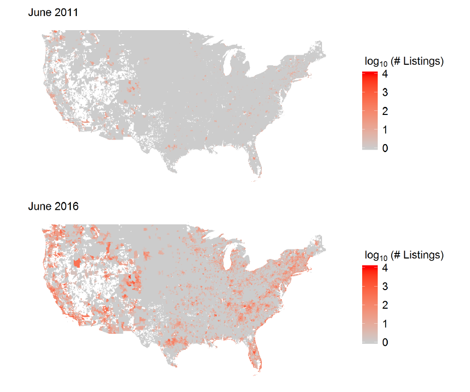
Figure 2: Map of Airbnb Listings by Zipcode, 2011-2016

Note: The ﬁgure shows the spatial distribution of Airbnb listings in June 2011 and June 2016,

where the number of listings is calculated using method 1 in Table 1. Listings are reported in logs,

and log listings is set to zero if there are zero listings. Geographic areas without zipcode boundary

information are colored white.

Electronic copy available at: https://ssrn.com/abstract=3006832

Figure 3: Total Number of Airbnb Listings (US, 2008-2016)

100,000

200,000

300,000

400,000

Jan 2008 Jan 2010 Jan 2012 Jan 2014 Jan 2016

Airbnb Supply

100,000

200,000

300,000

Jan 2008 Jan 2010 Jan 2012 Jan 2014 Jan 2016

Airbnb Supply

250,000

500,000

750,000

1,000,000

Jan 2008 Jan 2010 Jan 2012 Jan 2014 Jan 2016

Airbnb Supply

(a) (b) (a)

Note: This ﬁgure plots the number of Airbnb listings over time, using each of the 3 methods

described in Table 1: (a) method 1 – cumulative supply, (b) method 2 – TTL = 3 months, (c)

method 3 – TTL = 6 months.

Figure 4: Testing the IV Operating Assumption

●

100

0 25 50 75 100

Google trends

Difference in Airbnb listings between

high− and low−touristness zipcodes

Note: This ﬁgure plots the diﬀerence in the number of Airbnb listings for high- and low-touristiness

zipcodes over the Google trend values. We use the sample median value of touristiness to create

two equally sized groups of high- and low-touristiness zipcodes.

Electronic copy available at: https://ssrn.com/abstract=3006832

Figure 5: Trends in Zillow Home Value Index by “Touristiness” of Zipcode

-.1 0 .1 .2 .3

log ZHVI (Baseline: Jan 2011)

2009 2010 2011 2012 2013 2014 2015 2016 2017

1 2 3 4

Quartile for touristiness in 2010

Zillow Home Value Index

-.02 -.01 0 .01 .02

Residuals (Baseline: Jan 2011)

2009 2010 2011 2012 2013 2014 2015 2016 2017

1 2 3 4

Quartile for touristiness in 2010

Zillow Home Value Index (residuals)

Note: The top panel plots the ZHVI index, normalized to January 2011=0, averaged within diﬀerent groups

of zipcodes based on their level of “touristiness” in 2010. Touristiness is measured as the number of estab-

lishments in the food services and accommodations sector (NAICS code 72) in 2010, and the zipcodes are

separated into four equally sized groups. The bottom panel plots the residuals from a regression of the ZHVI

on zipcode ﬁxed eﬀects and CBSA-month ﬁxed eﬀects.

Electronic copy available at: https://ssrn.com/abstract=3006832

Figure 6: Christian and Barrett (2017) Exercise Results

-20 -10 0 10 20 30

coefficient

0.05

0.1

0.15

0.2

0.25

density

DV: ln ZRI

Main Effect (coefficient)

CB coefs 2SLS coef = 0.044

-100 -50 0 50 100

coefficient

0.02

0.04

0.06

0.08

density

DV: ln ZHVI

Main Effect (coefficient)

CB coefs 2SLS coef = 0.077

-4 -3 -2 -1 0 1 2

coefficient

0.5

1.5

density

DV: ln ZHVI/ZRI

Main Effect (coefficient)

CB coefs 2SLS coef = 0.032

0 5 10 15

t-stat

0.2

0.4

0.6

0.8

density

DV: ln ZRI

Main Effect (t-stat)

CB t-stat 2SLS t-stat = 14.7

0 5 10 15

t-stat

0.2

0.4

0.6

0.8

density

DV: ln ZHVI

Main Effect (t-stat)

CB t-stat 2SLS t-stat = 15.4

0 2 4 6 8 10

t-stat

0.5

1.5

density

DV: ln ZHVI/ZRI

Main Effect (t-stat)

CB t-stat 2SLS t-stat = 8.0

Note: This ﬁgure shows the distribution of the t-statistics for both the main coeﬃcient on Airbnb and the

coeﬃcient on the interaction term Airbnb × oorate for our three dependent variables using the Christian and

Barrett (2017) randomized regressors described in Section 5.1.

Electronic copy available at: https://ssrn.com/abstract=3006832

Figure 7: Google Trends Index for Related Websites (Worldwide, 2008-2019)

0 20 40 60 80 100

Google Trends Index

2008 2010 2012 2014 2016 2018 2020

Airbnb VRBO

HomeAway TripAdvisor

Expedia

Note: Monthly Google Trends index for various tourism related websites, from any searches world-

wide. Google Trends data are normalized so that the highest search volume over all the compared

terms and time-periods is equal to 100.

Electronic copy available at: https://ssrn.com/abstract=3006832

Table 2: Size of Airbnb Relative to the Housing Stock (zipcodes, 100 largest CBSAs)

p10 p25 p50 p75 p90

June 2011

Airbnb Listings 0 0 0 2 7

Housing Units 1,058 2,813 7,437 12,829 18,037

Airbnb Listings as a Percentage of

Total Housing Units .00 .00 .00 .02 .09

Renter-occupied Units .00 .00 .00 .06 .33

Vacant Units .00 .00 .00 .20 .92

Vacant-for-rent Units .00 .00 .00 1.01 5.06

June 2016

Airbnb Listings 1 4 13 44 144

Housing Units 1,097 2,926 7,610 13,219 18,443

Airbnb Listings as a Percentage of

Total Housing Units .03 .08 .21 .60 1.88

Renter-occupied Units .13 .33 .87 2.50 7.31

Vacant Units .37 .99 2.63 7.19 20.00

Vacant-for-rent Units 1.72 4.65 13.70 42.80 129.00

Note: This table reports the size of Airbnb relative to the housing stock by zipcodes for the 100 largest

CBSAs as measured by 2010 population. The number of Airbnb listings is calculated using method 1 in

Table 1. Data on housing stocks, occupancy characteristics, and vacancies come from ACS zipcode level

5-year estimates.

Electronic copy available at: https://ssrn.com/abstract=3006832

Table 3: IV Validity Check: Correlation Between Instrument and Rents/Prices in Zipcodes Without

Airbnb

Sample: Zipcodes Sample: Zipcodes Sample: Propensity-Score

w/o Airbnb ever w/ some Airbnb matched sample w/ Airbnb

(1) (2) (3) (4) (5) (6)

DV: ln ZRI DV: ln ZHVI DV: ln ZRI DV: ln ZHVI DV: ln ZRI DV: ln ZHVI

× h

i,2010

−1.63E−06 −3.92E−06 3.17E−06*** 5.38E−06*** 9.88E−06*** 8.77E−06*

(3.17E−06) (4.48E−06) (2.22E−07) (3.43E−07) (3.46E−06) (4.52E−06)

ln Population 0.011 0.045*** 0.055*** 0.087*** 0.052*** 0.077***

(0.013) (0.016) (0.007) (0.011) (0.019) (0.029)

ln Median HH Income −0.002 −0.001 0.027*** 0.017* 0.013 0.008

(0.011) (0.016) (0.006) (0.009) (0.015) (0.023)

College Share 0.054* 0.120*** 0.057*** 0.058*** 0.052 −0.053

(0.032) (0.038) (0.014) (0.020) (0.034) (0.063)

Employment Rate 0.045 −0.017 0.044*** 0.126*** 0.011 0.133**

(0.031) (0.033) (0.015) (0.023) (0.036) (0.060)

Zipcode FE Yes Yes Yes Yes Yes Yes

CBSA-year-month FE Yes Yes Yes Yes Yes Yes

Observations 61854 50875 587141 520797 51800 42082

0.979 0.994 0.992 0.996 0.982 0.993

Signiﬁcance levels: * p<0.1, ** p<0.05, *** p<0.01

Note: This table reports regression results when outcomes of interest are regressed on the instrumental variable

directly for three samples of zipcodes: 1) zipcodes that were never observed to have any Airbnb listings, 2) zipcodes

that were observed at some point to have Airbnb listings, and 3) zipcodes that had Airbnb listings and were propensity-

score matched to zipcodes that did not have Airbnb listings. Because zipcode demographic characteristics are not

available at a monthly frequency, zipcode-month measures for household income, population, college share, and

employment rate are interpolated from the 2011 thru 2016 ACS 5-year estimates. Clustered standard errors at the

zipcode level are reported in parenthesis.

Electronic copy available at: https://ssrn.com/abstract=3006832

Table 4: Comparing Airbnb and Non-Airbnb Zipcodes

Sample: Zipcodes Sample: Zipcodes Sample: Propensity-Score

w/o Airbnb w/ some Airbnb matched sample w/ Airbnb

Touristiness 7.40 43.73*** 7.34

ln Median Income 10.90 11.05*** 10.90

ln Population 8.25 9.44*** 8.28

College Share 0.19 0.34*** 0.19

Employment Rate 0.72 0.73*** 0.72

# Zipcodes 999 9356 999

Note: This table reports mean zipcode characteristics from three samples: 1) zipcodes that were never observed to

have any Airbnb listings, 2) zipcodes that were observed at some point to have Airbnb listings, and 3) zipcodes that

had Airbnb listings and were propensity-score matched to zipcodes that did not have Airbnb listings. *** indicates

that the diﬀerence in means compared to the non-Airbnb sample is statistically signiﬁcant with p<0.01.

Table 5: The Eﬀect of Airbnb on Rental Rates

(1) (2) (3) (4) (5) (6)

ln Airbnb Listings 0.098*** 0.008*** 0.022*** 0.021*** 0.046*** 0.044***

(0.002) (0.001) (0.001) (0.001) (0.003) (0.003)

. . . × Owner-occupancy Rate (2010) −0.023*** −0.022*** −0.038*** −0.036***

(0.002) (0.002) (0.003) (0.003)

ln Population 0.050*** 0.042***

(0.007) (0.007)

ln Median HH Income 0.021*** 0.017***

(0.005) (0.006)

College Share 0.063*** 0.057***

(0.013) (0.013)

Employment Rate 0.048*** 0.036***

(0.014) (0.014)

Zipcode FE No Yes Yes Yes Yes Yes

CBSA-year-month FE No Yes Yes Yes Yes Yes

Instrumental Variable No No No No Yes Yes

Observations 649841 649841 649841 649697 649841 649697

0.169 0.991 0.991 0.991 0.991 0.991

Kleinbergen-Paap F Statistic 820.0 807.0

Signiﬁcance levels: * p<0.1, ** p<0.05, *** p<0.01

Note: The number of Airbnb listings is calculated using method 1 in Table 1. To avoid taking the log of a zero,

one is added to the number of Airbnb listings before taking logs. The instrumental variables are g

× h

i,2010

and

× h

i,2010

× oorate

ict

. Because zipcode demographic characteristics are not available at a monthly frequency,

zipcode-month measures for household income, population, college share, and employment rate are interpolated from

the 2011 thru 2016 ACS 5-year estimates. Clustered standard errors at the zipcode level are reported in parenthesis.

All variables are seasonally adjusted.

Electronic copy available at: https://ssrn.com/abstract=3006832

Table 6: The Eﬀect of Airbnb on House Prices

(1) (2) (3) (4) (5) (6)

ln Airbnb Listings 0.175*** 0.009*** 0.040*** 0.038*** 0.080*** 0.077***

(0.004) (0.001) (0.002) (0.002) (0.005) (0.005)

. . . × Owner-occupancy Rate (2010) −0.048*** −0.046*** −0.074*** −0.071***

(0.003) (0.003) (0.006) (0.006)

ln Population 0.077*** 0.063***

(0.010) (0.010)

ln Median HH Income 0.012 0.005

(0.008) (0.008)

College Share 0.073*** 0.061***

(0.018) (0.018)

Employment Rate 0.099*** 0.070***

(0.020) (0.020)

Zipcode FE No Yes Yes Yes Yes Yes

CBSA-year-month FE No Yes Yes Yes Yes Yes

Instrumental Variable No No No No Yes Yes

Observations 572858 572858 572858 572805 572858 572805

0.188 0.996 0.996 0.996 0.996 0.996

Kleinbergen-Paap F Statistic 661.9 646.7

Signiﬁcance levels: * p<0.1, ** p<0.05, *** p<0.01

Note: The number of Airbnb listings is calculated using method 1 in Table 1. To avoid taking the log of a zero,

one is added to the number of Airbnb listings before taking logs. The instrumental variables are g

× h

i,2010

and

× h

i,2010

× oorate

ict

. Because zipcode demographic characteristics are not available at a monthly frequency,

zipcode-month measures for household income, population, college share, and employment rate are interpolated from

the 2011 thru 2016 ACS 5-year estimates. Clustered standard errors at the zipcode level are reported in parenthesis.

All variables are seasonally adjusted.

Electronic copy available at: https://ssrn.com/abstract=3006832

Table 7: The Eﬀect of Airbnb on Price-to-Rent Ratio

(1) (2) (3) (4) (5) (6)

ln Airbnb Listings 0.077*** 0.002** 0.016*** 0.015*** 0.032*** 0.032***

(0.002) (0.001) (0.002) (0.002) (0.004) (0.004)

. . . × Owner-occupancy Rate (2010) −0.022*** −0.022*** −0.032*** −0.032***

(0.003) (0.003) (0.005) (0.005)

ln Population 0.030*** 0.025**

(0.010) (0.010)

ln Median HH Income −0.013 −0.016*

(0.009) (0.009)

College Share 0.011 0.006

(0.019) (0.019)

Employment Rate 0.046** 0.034

(0.022) (0.022)

Zipcode FE No Yes Yes Yes Yes Yes

CBSA-year-month FE No Yes Yes Yes Yes Yes

Instrumental Variable No No No No Yes Yes

Observations 537157 537142 537142 537089 537142 537089

0.154 0.979 0.979 0.979 0.979 0.979

Kleinbergen-Paap F Statistic 629.8 616.9

Signiﬁcance levels: * p<0.1, ** p<0.05, *** p<0.01

Note: The number of Airbnb listings is calculated using method 1 in Table 1. To avoid taking the log of a zero,

one is added to the number of Airbnb listings before taking logs. The instrumental variables are g

× h

i,2010

and

× h

i,2010

× oorate

ict

. Because zipcode demographic characteristics are not available at a monthly frequency,

zipcode-month measures for household income, population, college share, and employment rate are interpolated from

the 2011 thru 2016 ACS 5-year estimates. Clustered standard errors at the zipcode level are reported in parenthesis.

All variables are seasonally adjusted.

Electronic copy available at: https://ssrn.com/abstract=3006832

Table 8: Controlling for Measures of Tourism Demand

DV: ln ZRI DV: ln ZHVI

(1) (2) (3) (4) (5) (6) (7) (8) (9) (10)

ln Airbnb Listings 0.040*** 0.044*** 0.044*** 0.044*** 0.044*** 0.071*** 0.078*** 0.077*** 0.085*** 0.046***

(0.003) (0.003) (0.003) (0.003) (0.006) (0.005) (0.005) (0.005) (0.006) (0.008)

. . . × Owner-occupancy Rate (2010) −0.034*** −0.035*** −0.036*** −0.036*** −0.036*** −0.069*** −0.071*** −0.071*** −0.076*** −0.056***

(0.003) (0.003) (0.003) (0.003) (0.004) (0.006) (0.006) (0.006) (0.007) (0.006)

ln Population 0.043*** 0.044*** 0.041*** 0.042*** 0.042*** 0.069*** 0.071*** 0.063*** 0.062*** 0.073***

(0.007) (0.007) (0.007) (0.007) (0.007) (0.010) (0.010) (0.010) (0.010) (0.010)

ln Median HH Income 0.018*** 0.018*** 0.018*** 0.017*** 0.017*** 0.003 0.004 0.005 0.005 0.006

(0.006) (0.006) (0.006) (0.006) (0.006) (0.008) (0.008) (0.008) (0.008) (0.008)

College Share 0.052*** 0.055*** 0.056*** 0.057*** 0.057*** 0.053*** 0.057*** 0.061*** 0.060*** 0.066***

(0.014) (0.014) (0.013) (0.013) (0.013) (0.018) (0.019) (0.018) (0.018) (0.018)

Employment Rate 0.038*** 0.038*** 0.037*** 0.036*** 0.036** 0.079*** 0.078*** 0.071*** 0.067*** 0.087***

(0.014) (0.014) (0.014) (0.014) (0.014) (0.020) (0.020) (0.020) (0.020) (0.020)

Food & Accommodations Estabs. 3.48E−04*** 5.83E−04***

(7.15E−05) (1.25E−04)

ln Hotel Occupancy 4.83E−04*** 4.31E−04

(1.83E−04) (2.77E−04)

ln Airport Travelers (arrivals) 3.36E−04*** 1.37E−04

(1.18E−04) (1.79E−04)

# Trip Advisor Reviews 1.38E−07 −3.58E−05***

(3.55E−06) (1.08E−05)

t × h

i,2010

−7.94E−08 3.58E−06***

(9.31E−07) (1.07E−06)

Zipcode FE Yes Yes Yes Yes Yes Yes Yes Yes Yes Yes

CBSA-year-month FE Yes Yes Yes Yes Yes Yes Yes Yes Yes Yes

Instrumental Variable Yes Yes Yes Yes Yes Yes Yes Yes Yes Yes

Observations 639400 639400 648905 649697 649697 564157 564157 572085 572805 572805

0.991 0.991 0.991 0.991 0.991 0.996 0.996 0.996 0.996 0.996

Kleinbergen-Paap F Statistic 650.0 761.5 802.8 791.9 167.1 516.1 611.9 642.5 579.2 218.3

Signiﬁcance levels: * p<0.1, ** p<0.05, *** p<0.01

Note: The number of Airbnb listings is calculated using method 1 in Table 1. To avoid taking the log of a zero,

one is added to the number of Airbnb listings before taking logs. The instrumental variables are g

× h

i,2010

and

× h

i,2010

× oorate

ict

. Because zipcode demographic characteristics are not available at a monthly frequency,

zipcode-month measures for household income, population, college share, and employment rate are interpolated from

the 2011 thru 2016 ACS 5-year estimates. Clustered standard errors at the zipcode level are reported in parenthesis.

All variables are seasonally adjusted.

Electronic copy available at: https://ssrn.com/abstract=3006832

Table 9: Eﬀect Magnitudes for 10 Largest CBSAs

Year-over-Year Airbnb Year-over-Year

Contribution Growth

CBSA Rent Price Rent Price

Top 100 CBSAs 0.59% 0.82% 3.18% 5.70%

New York-Newark-Jersey City, NY-NJ-PA 0.60% 0.83% 3.64% 3.55%

Los Angeles-Long Beach-Anaheim, CA 1.14% 1.79% 4.92% 9.66%

Chicago-Naperville-Elgin, IL-IN-WI 0.34% 0.44% 2.25% 3.98%

Dallas-Fort Worth-Arlington, TX 0.70% 1.01% 4.18% 8.21%

Miami-Fort Lauderdale-West Palm Beach, FL 1.02% 1.51% 4.51% 11.72%

Philadelphia-Camden-Wilmington, PA-NJ-DE-MD 0.54% 0.73% 1.94% 2.05%

Houston-The Woodlands-Sugar Land, TX 0.95% 1.37% 4.67% 8.34%

Washington-Arlington-Alexandria, DC-VA-MD-WV 0.70% 0.96% 1.28% 4.41%

Atlanta-Sandy Springs-Roswell, GA 0.75% 1.07% 3.11% 8.42%

Detroit-Warren-Dearborn, MI 0.16% 0.21% 2.41% 8.54%

Note: Airbnb contribution is calculated as

β + ˆγoorate

ic,2010

multiplied by the median year-over-year growth

in log Airbnb listings for each zipcode, and then taken at the median zipcode. Estimates from columns 6 of

Tables 5 and 6 are used.

Electronic copy available at: https://ssrn.com/abstract=3006832

Table 10: The Eﬀect of Airbnb on Housing Supply

(1) (2) (3) (4)

ln Vacant Seasonal ln Vacant For-Rent ln Rental Stock ln Housing Stock

ln Airbnb Listings 0.078*** −0.048* −0.036*** −0.002

(0.025) (0.025) (0.006) (0.002)

. . . × Owner-occupancy Rate (2010) −0.018 0.045* 0.053*** −0.002

(0.032) (0.027) (0.005) (0.003)

ln Population −0.212*** −0.225*** 0.871*** 0.547***

(0.055) (0.079) (0.032) (0.019)

ln Median HH Income 0.051 0.151*** −0.457*** −0.074***

(0.046) (0.055) (0.026) (0.011)

College Share −0.016 −0.052 −0.177*** 0.100***

(0.116) (0.152) (0.066) (0.024)

Employment Rate 0.093 −0.465*** 0.315*** 0.146***

(0.123) (0.152) (0.068) (0.033)

Zipcode FE Yes Yes Yes Yes

Year FE Yes Yes Yes Yes

Instrumental Variable Yes Yes Yes Yes

Observations 49282 49580 61435 61720

0.913 0.927 0.993 0.999

Kleinbergen-Paap F Statistic 742.4 587.2 1082.9 1099.4

Signiﬁcance levels: * p<0.1, ** p<0.05, *** p<0.01

Note: Deﬁnitions of the dependent variables are given in Section 6.4. The number of Airbnb listings is calculated

using method 1 in Table 1. To avoid taking the log of a zero, one is added to the number of Airbnb listings before

taking logs. Clustered standard errors at the zipcode level are reported in parentheses.

Electronic copy available at: https://ssrn.com/abstract=3006832

For Online Publication: Appendix

A Monte Carlo Simulation of Placebo Test

In Section 5.1, we describe the test proposed by Christian and Barrett (2017) (CB exercise) in

which a randomized regressor is constructed by keeping the identity of which zipcodes had non-zero

Airbnb listings but swapping the actual number of Airbnb listings across zipcodes. The randomized

regressor preserves the overall time trends in the number of Airbnb listings but randomizes the

intensive margin of Airbnb growth experienced by each zipcode, thus eliminating the impact of

touristiness on the intensive margin of Airbnb listings. If the results are primarily driven by

spurious time trends that interact with the extensive margin of Airbnb listings, then the exercise

will produce 2SLS estimates that continue to be positive and statistically signiﬁcant. This is what

happens when Christian and Barrett (2017) apply their exercise to the Nunn and Qian (2014)

instrument for U.S. Food Aid, which they were critiquing. In our case, if the eﬀect of touristiness

on the intensive margin of Airbnb listings is what really matters, then the ﬁrst-stage will become

very weak when regressing the randomized regressor on the instrument. The weak ﬁrst stage results

in a high variance of second stage estimates when performing 2SLS using the randomized regressor

and statistically insigniﬁcant estimates.

Here, we demonstrate using a Monte Carlo simulation with an instrument that is known to

be valid. We will show that the CB exercise leads to a large variance of point estimates that are

statistically insigniﬁcant. Consider a model in which X

is our endogenous explanatory regressor

and Y

is our outcome of interest. The causal relation is:

= βX

+ 

(3)

and X

is a non-negative regressor given by:











+ γ

× G

+ ν

if c

= 0

0 if c

= 1

(4)

The censoring indicator, c

, controls whether X

is zero. For simplicity, we assume that γ

is large

Electronic copy available at: https://ssrn.com/abstract=3006832

enough so that X

> 0 when c

= 0. Crucially, we assume that:

P (c

= 1) =

1 + exp(3 + ν

)

(5)

so that c

, which controls the extensive margin of X

, is exogenous to H

× G

but endogenous to

. c

is analogous to whether the zipcode i had zero Airbnb listings in time t.

To induce correlation between X

and 

, which necessitates an instrument, we introduce a

spurious time trend D

, which interacts with H

, that simultaneously aﬀects ν

and 

= θD

× H

+ ξ

(6)



= φD

× H

+ η

(7)

We simulate the above system using β = 1, γ

= 10, γ

= θ = φ = 1 . We draw H

, G

, D

, ξ

and η

from iid standard normal distributions, which implies that E [

× G

] = 0 and thus

= H

× G

is a valid instrument for X

To summarize this model, Y

is analogous to rent, X

is analogous to Airbnb, H

is analogous

to touristiness, and G

is analogous to the Google trends. In the Monte Carlo, X

is endogenous

through the correlation between ν

and 

, which is driven by a spurious time trend that interacts

with touristiness: D

× H

OLS estimation of equation (3) results in a biased estimate of

OLS

= 1.151

∗∗∗

(0.002). 2SLS

estimation of equation (3) using Z

= H

× G

as the instrument for X

results in an estimate of

= 0.993

∗∗∗

(0.007). The true parameter, β = 1, is contained in the 95% conﬁdence interval of

the 2SLS estimate, which is expected since Z

is known to be a valid instrument.

We then perform the CB exercise using the simulated data, which essentially amounts to ran-

domly swapping X

among the i’s with c

= 0, without changing any other variables. We do this

500 times. The top left panel of Figure 8 plots the density of the resulting estimates along with

the baseline 2SLS estimate from the non-randomized Monte-Carlo data. The variance of the CB

estimates is very large and the 2SLS estimate for β as well as the true parameter are well within

the 5th-95th-percentile-range of the CB estimates. For comparison, in the top right panel of Figure

8, we reproduce the same plot using the data from our paper when the dependent variable is ln

Electronic copy available at: https://ssrn.com/abstract=3006832

ZRI. We can observe that the results of the CB exercise using our data and our instrument are

very similar to those obtained with a valid simulated instrument.

The bottom left panel of Figure 8 then shows the density of the t-statistics of the CB estimates

using the Monte Carlo data along with the t-stat of the baseline 2SLS estimate. In the bottom

right panel, we reproduce the same plot using the data from our paper. As before, we observe that

the results of the CB exercise using the data from our paper is very simlar to those obtained in the

Monte Carlo with a valid simulated instrument; that is, the t-stats in the CB exercise are small and

centered around zero, whereas the t-stat of the main 2SLS estimate is large and implies statistical

signiﬁcance.

Finally, we use our Monte Carlo simulation to explore what happens when we use an invalid

instrument. We note that

= D

× H

will be correlated with 

through a spurious time trend

and is thus not a valid instrument. Indeed, when we perform 2SLS using

as an instrument for

, we estimate

invalidIV

= 1.671

∗∗∗

(0.006), which is not close to the true parameter. Moreover,

, by design, aﬀects the extensive margin of X

, and therefore we expect to ﬁnd statistically

signiﬁcant estimates when we perform the CB randomization. The top left panel of Figure 9 shows

the resulting coeﬃcient estimates from the CB exercise, and indeed they are shifted to the right of

main estimate with non-randomized data. Moreover, the bottom left panel shows the t-stats of the

CB exercise and shows that all of the CB estimates are statistically signiﬁcant. These results are

consistent with what Christian and Barrett (2017) show in Figure 6 of their paper (reproduced in

the top right panel of Figure 9), which they use as an argument for the invalidity of the instrument

they are critiquing.

Given these results, our conclusion is that, given a valid instrument, the CB exercise should

produce estimates with a very large variance that encompasses the baseline estimate, and such

estimates should be statistically insigniﬁcant. These are exactly the results we obtain using our

data and instrument.

Electronic copy available at: https://ssrn.com/abstract=3006832

B Robustness Checks

Alternative measures of Airbnb supply

In this Appendix, we show that our results are robust to a number of speciﬁcation and sensitivity

checks. First, we show that our main results are robust to alternative methods of calculating Airbnb

supply. As discussed in Section 4, we can never know the exact number of active Airbnb listings at

any given point in time, and we therefore construct Airbnb supply using the three methods of Table

1. In Table 11, we report regression results when methods 2 and 3 are used to measure Airbnb

supply instead of method 1. The results are barely changed, which is not surprising given the high

correlation between the three measures, despite level diﬀerences.

In our main results, we use a log-log speciﬁcation to measure the eﬀect of Airbnb listings

on house prices and rental rates because such speciﬁcation provides us with easily interpretable

coeﬃcients in the form of elasticity that is often used in competitive settings and has been used

in the past in the context of Airbnb (Zervas et al., 2017; Farronato and Fradkin, 2018). However,

as Zervas et al. (2017) observe, the log-log speciﬁcation implies constant elasticity, an assumption

that might not hold in our setting. To make sure that our results are not driven by the log-log

choice, we use an alternative speciﬁcation in which Airbnb

ict

in equation (2) is measured as the

number of Airbnb listings divided by the total occupied housing stock.

We call this measure

“Airbnb density.” One of the downsides of the log-density speciﬁcation is that Airbnb density is

extremely skewed

, and using g

× h

i,2010

as the instrument, the ﬁrst stage becomes very weak

and we fail to reject underidentiﬁcation.

We therefore report results using an augmented set of

instruments. First, we try g

× h

i,2010

/stock

i,2010

interacted with oorate

i,2010

, where stock

i,2010

the total occupied housing stock in 2010. Second, we try a third order polynomial of g

× h

i,2010

(our original instrument), interacted with oorate

i,2010

. Third, we try fully interacted second order

polynomials of g

, h

i,2010

, and oorate

i,2010

. We report the results in Table 12. The main results hold

qualitatively: (i) higher Airbnb density leads to higher house prices and rental rates, (ii) the eﬀect

is higher for house prices than for rental rates, and (iii) the eﬀect is decreasing in owner-occupancy

Data on total occupied housing stock is from ACS 5-year estimates from 2011 to 2016.

The skewness is 129.58 compared to a mean of 0.007 and variance of 0.06.

In the rent regression, an underidentiﬁcation test using the Kleibergen and Paap (2006) rk LM statistic fails to

reject underidentiﬁcation with a p-value of 0.6650.

Electronic copy available at: https://ssrn.com/abstract=3006832

rate. However, the coeﬃcients are somewhat sensitive to the choice of instruments. Thus, the

log-log speciﬁcation, which has proven to be very robust, remains our preferred speciﬁcation.

Finally, recall that in our main speciﬁcation we added one to the number of Airbnb listings to

avoid taking logs of zero. We now show that the results are robust to this choice. Table 13 reports

regression results when instead of adding one to the number of listings, we instead simply drop

all zipcode-year-month observations in which the number of listings is zero. We also try dropping

all observations where the number of listings is less than 5. The results remain qualitatively and

quantitatively similar to the main results, suggesting both that adding one to the number of Airbnb

listings does not aﬀect the results but also that the results are not primarily being driven by zipcodes

with very few Airbnb listings.

Heterogeneous eﬀects across subsamples

We now test whether the results are heterogeneous or homogeneous across various subsamples of

our data. We ﬁnd that the eﬀects may be heterogeneous but that the main qualitative result that

Airbnb has a positive eﬀect on prices and rents and is moderated by the owner-occupancy rate

holds across subsamples.

First, we test whether Airbnb has diﬀerent eﬀects by distance to the city-center. We run the

2SLS regressions for two subsamples: the sample of zipcodes below the median distance to the city

center, and the sample of zipcodes above the median distance to the city center, where the median

is taken within CBSA. The results are reported in Table 14. The qualitative results hold in both

the near and far samples, though it seems that the eﬀects are actually larger in the far group. This

conﬁrms that the results are not being solely driven by a few zipcodes close to downtown areas and

that home-sharing is having an impact even on zipcodes that are further from the city center.

Second, we test whether Airbnb has diﬀerent eﬀects in two time periods: 2011-2013 and 2014-

2016. The results are reported in Table 15. Again, the main qualitative results can be seen in

both time periods though the eﬀect of owner-occupancy rate seems to be a lot weaker in the earlier

period than in the later period, and the results on price-to-rent ratio are not signiﬁcant in the

earlier period. We speculate that this could be due to the possibility that Airbnb ﬁrst attracted

those users with spare rooms or houses not in the long-term market (i.e., vacation homes) and that

only recently did Airbnb become an attractive option for landlords that previously rented in the

Electronic copy available at: https://ssrn.com/abstract=3006832

long-term market.

Third, we repeat the regressions separately for the 30 largest CBSAs and for the CBSAs ranked

31-100 in terms of 2010 population. Table 16 reports the results. The qualitative results hold for

both samples, though the results are not statistically signiﬁcant in the rank 31-100 sample when

the dependent variable is price-to-rent ratio. The eﬀects of Airbnb appear to be stronger in the

larger cities, which could be driven by a number of factors, including diﬀerences in housing demand

and the tightness of the rental market.

Eﬀects on subsegments of the housing market

Now we test whether Airbnb has diﬀerent eﬀects on diﬀerent subsegments of the housing market.

In our main regressions, we used the ZRI and the ZHVI for our dependent variables, both of which

measure the median rent/home value for the stock of homes in a zipcode. Thus, the results do

not speak to whether or not Airbnb can have diﬀerential eﬀects on diﬀerent quality segments of

the housing market. To test this, we now run the regressions using six additional rent and price

measures. For rents, Zillow provides a separate index for rentals of multifamily and single-family

units. For prices, Zillow provides a separate house price index for homes with 1, 2, 3, and 4

bedrooms (including both condos and single-family detached units.) The results are reported in

Table 17. The results show that the eﬀects are not too diﬀerent across diﬀerent subsegments of the

housing market.

Additional tests

Now we show that our results are robust to the inclusion of the Google Trends index for other

tourism-based websites interacted with baseline touristiness. This is an extension of the controls

for tourism discussed in Section 6.2 and also addresses the extent to which our results reﬂect home-

sharing in total or primarily the eﬀect of Airbnb (though it is hard to fully separate as many listings

are cross-listed across multiple platforms and Google searches are not a perfect proxy for actual

usage.) Table 18 shows these results and shows that our results are robust to the inclusion of any

of these controls.

Finally, we show that our results are robust to using forward-looking measures of zipcode

demographics. This addresses the concern that house prices and rental rates adjust more quickly

Electronic copy available at: https://ssrn.com/abstract=3006832

than demographic composition. In Table 19, we control for contemporaneous, 1-year ahead, and

2-year ahead measures of demographic characteristics. The results are robust to either choice. Note

that when we use the 2-year ahead demographic variables, the results look more like the results

from the 2011-2013 sample in Table 15 because we only use data up to 2014 since our demographic

variables are only measured until 2016. Thus, the diﬀerences in controlling for 1-year ahead and

2-year ahead demographic variables can be attributed more to changes to the sample than the

choice of when to measure the demographics.

Electronic copy available at: https://ssrn.com/abstract=3006832

Figure 8: Monte Carlo Results for CB Exercise Using Valid Instrument, Compared with Our Paper

-2000 -1000 0 1000 2000 3000

coefficient

0.5

1.5

density

-3

MC Simulation w Valid Instrument

Estimated Coefficients

CB values Baseline value = 0.9928

-30 -20 -10 0 10 20 30 40

coefficient

0.05

0.1

0.15

0.2

0.25

density

Our data and instrument

DV:ZRI, Main Effect Coefficients

CB values Baseline value = 0.0440

0 50 100 150

t-stat

0.2

0.4

0.6

0.8

density

MC Simulation w Valid Instrument

t-stats

CB values Baseline value = 135.9055

-5 0 5 10 15

t-stat

0.2

0.4

0.6

0.8

density

Our data and instrument

DV:ZRI, Main Effect t-stats

CB values Baseline value = 14.6667

Note: The Christian and Barrett (2017) exercise is described in Section 5.1 of the paper and Appendix A.

The top left panel shows the distribution of CB estimates along with the main 2SLS estimate using the

non-randomized Monte Carlo data. The top right panel reproduces this using the data from the paper when

ln ZRI is the dependent variable. The bottom left panel shows the distribution of the t-stats of the CB

estimates along with the t-stat of the main 2SLS estimate using the non-randomized Monte Carlo data. The

bottom right panel reproduces this using data from the paper.

Electronic copy available at: https://ssrn.com/abstract=3006832

Figure 9: Monte Carlo Results for CB Exercise Using Invalid Instrument, Compared with Christian

and Barrett (2017)

1.6 1.8 2 2.2 2.4 2.6 2.8 3 3.2 3.4

coefficient

density

MC Simulation w Invalid Instrument

Estimated Coefficients

CB values Baseline value= 1.6712

50 100 150 200 250 300

t-stat

0.1

0.2

0.3

0.4

0.5

density

MC Simulation w Invalid Instrument

t-stats

CB values Baseline value= 292.1381

Christian and Barret (2017)

Figure 6 (Invalid Instrument)

Note: The Christian and Barrett (2017) exercise is described in Section 5.1 of the paper and Appendix A.

The top left panel shows the distribution of CB estimates along with the main 2SLS estimate using the non-

randomized Monte-Carlo data, when the instrument is not valid (the Monte Carlo simulation is described

in Appendix A). The bottom left panel shows the distribution of the t-stats. The top right panel shows the

distribution of CB estimates from Christian and Barrett (2017) produced using data from Nunn and Qian

(2014). The red line labeled “NQ” is the main 2SLS estimate from Nunn and Qian (2014).

Electronic copy available at: https://ssrn.com/abstract=3006832

Table 11: 2SLS Results with Alternative Measures of Airbnb Supply

Airbnb Measure: Method 2 Airbnb Measure: Method 3

(1) (2) (3) (4) (5) (6)

DV: ln ZRI DV: ln ZHVI DV: ln ZHVI/ZRI DV: ln ZRI DV: ln ZHVI DV: ln ZHVI/ZRI

ln Airbnb Listings 0.048*** 0.088*** 0.037*** 0.049*** 0.088*** 0.036***

(0.003) (0.006) (0.005) (0.003) (0.006) (0.005)

. . . × Owner-occupancy Rate (2010) −0.040*** −0.083*** −0.038*** −0.041*** −0.085*** −0.038***

(0.004) (0.008) (0.006) (0.004) (0.008) (0.006)

ln Population 0.045*** 0.067*** 0.026** 0.044*** 0.066*** 0.026**

(0.007) (0.010) (0.010) (0.007) (0.010) (0.010)

ln Median HH Income 0.015*** 0.000 −0.018** 0.016*** 0.002 −0.017*

(0.006) (0.008) (0.009) (0.006) (0.008) (0.009)

College Share 0.053*** 0.052*** 0.002 0.055*** 0.056*** 0.004

(0.013) (0.018) (0.019) (0.013) (0.018) (0.019)

Employment Rate 0.035** 0.065*** 0.032 0.035** 0.066*** 0.032

(0.014) (0.020) (0.022) (0.014) (0.020) (0.022)

Zipcode FE Yes Yes Yes Yes Yes Yes

CBSA-year-month FE Yes Yes Yes Yes Yes Yes

Instrumental Variable Yes Yes Yes Yes Yes Yes

Observations 649697 572805 537089 649697 572805 537089

0.991 0.996 0.979 0.991 0.996 0.979

Kleibergen-Paap F Statistic 916.3 718.8 704.4 893.7 700.2 686.5

Signiﬁcance levels: * p<0.1, ** p<0.05, *** p<0.01

Note: The number of Airbnb listings is calculated using either method 1 or method 2 in Table 1. To avoid taking

the log of a zero, one is added to the number of Airbnb listings before taking logs. The instrumental variables

are g

× h

i,2010

and g

× h

i,2010

× oorate

ict

. Because zipcode demographic characteristics are not available at a

monthly frequency, zipcode-month measures for household income, population, college share, and employment rate

are interpolated from the 2011 thru 2016 ACS 5-year estimates. Clustered standard errors at the zipcode level are

reported in parenthesis. All variables are seasonally adjusted.

Electronic copy available at: https://ssrn.com/abstract=3006832

Table 12: 2SLS Results for Log-Density Speciﬁcations

Instrument Set 1 Instrument Set 2 Instrument Set 3

(1) (2) (3) (4) (5) (6) (7) (8) (9)

DV: ln ZRI DV: ln ZHVI DV: ln ZHVI/ZRI DV: ln ZRI DV: ln ZHVI DV: ln ZHVI/ZRI DV: ln ZRI DV: ln ZHVI DV: ln ZHVI/ZRI

Airbnb Density 1.003*** 2.525*** 1.520*** 1.891*** 3.606*** 1.685*** 1.569*** 2.658*** 1.058***

(0.219) (0.310) (0.330) (0.218) (0.373) (0.284) (0.185) (0.322) (0.270)

. . . × Owner-occupancy Rate (2010) −1.102* −3.874*** −3.070*** −3.894*** −6.693*** −3.134*** −2.549*** −3.440*** −1.644**

(0.605) (0.888) (0.989) (0.698) (1.118) (0.731) (0.555) (0.906) (0.679)

ln Population 0.054*** 0.064*** 0.010 0.034*** 0.041** 0.011 0.045*** 0.070*** 0.023*

(0.008) (0.013) (0.015) (0.011) (0.016) (0.012) (0.008) (0.013) (0.012)

ln Median HH Income 0.014** −0.002 −0.016* 0.008 −0.006 −0.018** 0.010* −0.005 −0.016*

(0.006) (0.008) (0.010) (0.008) (0.009) (0.009) (0.006) (0.009) (0.009)

College Share 0.053*** 0.045** 0.002 0.068*** 0.039* −0.001 0.058*** 0.042** −0.001

(0.015) (0.018) (0.019) (0.019) (0.021) (0.019) (0.014) (0.020) (0.019)

Employment Rate 0.044*** 0.097*** 0.053** 0.053*** 0.111*** 0.049** 0.046*** 0.087*** 0.044**

(0.015) (0.021) (0.023) (0.016) (0.022) (0.022) (0.015) (0.022) (0.022)

Zipcode FE Yes Yes Yes Yes Yes Yes Yes Yes Yes

CBSA-year-month FE Yes Yes Yes Yes Yes Yes Yes Yes Yes

Instrumental Variable Yes Yes Yes Yes Yes Yes Yes Yes Yes

Observations 613245 538990 504260 613245 538990 504260 613245 538990 504260

0.991 0.996 0.979 0.990 0.996 0.979 0.991 0.996 0.979

Kleibergen-Paap F Statistic 15.26 10.75 9.347 5.797 5.813 5.666 9.369 10.27 10.19

Signiﬁcance levels: * p<0.1, ** p<0.05, *** p<0.01

Note: The number of Airbnb listings is calculated using method 1 in Table 1, and is then divided by the total occupied

housing stock to calculate “Airbnb Density”. “Instrument Set 1” is g

× h

i,2010

/stock

i,2010

interacted with oorate

i,2010

“Instrument Set 2” is a third order polynomial of g

× h

i,2010

(our original instrument), interacted with oorate

i,2010

“Instrument Set 3” is a fully interacted second order polynomial of g

, h

i,2010

, and oorate

i,2010

. Clustered standard

errors at the zipcode level are reported in parenthesis. All variables are seasonally adjusted.

Electronic copy available at: https://ssrn.com/abstract=3006832

Table 13: 2SLS Results When Dropping Observations with Low Listings

Drop obs w/ 0 listings Drop obs w/ <5 listings

(1) (2) (3) (4) (5) (6)

DV: ln ZRI DV: ln ZHVI DV: ln ZHVI/ZRI DV: ln ZRI DV: ln ZHVI DV: ln ZHVI/ZRI

ln Airbnb Listings 0.049*** 0.092*** 0.041*** 0.034** 0.080*** 0.045**

(0.006) (0.010) (0.009) (0.014) (0.022) (0.020)

. . . × Owner-occupancy Rate (2010) −0.041*** −0.085*** −0.040*** −0.043*** −0.097*** −0.050***

(0.004) (0.007) (0.005) (0.005) (0.009) (0.008)

ln Population 0.037*** 0.046*** 0.006 0.006 0.012 0.011

(0.010) (0.015) (0.016) (0.013) (0.021) (0.020)

ln Median HH Income 0.035*** 0.011 −0.021 0.039*** 0.023 −0.009

(0.008) (0.012) (0.013) (0.009) (0.015) (0.016)

College Share 0.069*** 0.044 −0.019 0.095*** 0.073* −0.018

(0.018) (0.028) (0.027) (0.024) (0.041) (0.040)

Employment Rate 0.011 0.071** 0.044 0.029 0.102** 0.029

(0.020) (0.031) (0.031) (0.030) (0.045) (0.044)

Zipcode FE Yes Yes Yes Yes Yes Yes

CBSA-year-month FE Yes Yes Yes Yes Yes Yes

Instrumental Variable Yes Yes Yes Yes Yes Yes

Observations 444992 396821 380148 272298 245181 236996

0.993 0.996 0.983 0.995 0.997 0.986

Kleinbergen-Paap F Statistic 150.3 119.4 119.6 44.82 38.44 38.97

Signiﬁcance levels: * p<0.1, ** p<0.05, *** p<0.01

Note: The number of Airbnb listings is calculated using method 1 in Table 1. The instrumental variables are g

×h

i,2010

and g

× h

i,2010

× oorate

ict

. Because zipcode demographic characteristics are not available at a monthly frequency,

zipcode-month measures for household income, population, college share, and employment rate are interpolated from

the 2011 thru 2016 ACS 5-year estimates. Clustered standard errors at the zipcode level are reported in parenthesis.

All variables are seasonally adjusted.

Electronic copy available at: https://ssrn.com/abstract=3006832

Table 14: 2SLS Results by Distance to City Center

Zipcodes near city center Zipcodes far from city center

(1) (2) (3) (4) (5) (6)

DV: ln ZRI DV: ln ZHVI DV: ln ZHVI/ZRI DV: ln ZRI DV: ln ZHVI DV: ln ZHVI/ZRI

ln Airbnb Listings 0.030*** 0.058*** 0.027*** 0.059*** 0.098*** 0.036***

(0.003) (0.006) (0.006) (0.005) (0.008) (0.006)

. . . × Owner-occupancy Rate (2010) −0.022*** −0.048*** −0.024*** −0.052*** −0.098*** −0.041***

(0.004) (0.007) (0.007) (0.005) (0.009) (0.007)

ln Population 0.036*** 0.056*** 0.017 0.051*** 0.068*** 0.029**

(0.010) (0.013) (0.014) (0.010) (0.014) (0.015)

ln Median HH Income 0.014** −0.002 −0.016 0.021** 0.018 −0.011

(0.007) (0.010) (0.011) (0.009) (0.012) (0.014)

College Share 0.046*** 0.037 0.014 0.070*** 0.086*** −0.002

(0.017) (0.024) (0.027) (0.020) (0.028) (0.029)

Employment Rate 0.036** 0.050** 0.003 0.042** 0.073** 0.051

(0.018) (0.024) (0.028) (0.021) (0.032) (0.033)

Zipcode FE Yes Yes Yes Yes Yes Yes

CBSA-year-month FE Yes Yes Yes Yes Yes Yes

Instrumental Variable Yes Yes Yes Yes Yes Yes

Observations 317636 275627 255794 331959 297034 281079

0.991 0.996 0.977 0.991 0.996 0.981

Kleinbergen-Paap F Statistic 465.1 376.2 365.5 322.0 265.6 252.4

Signiﬁcance levels: * p<0.1, ** p<0.05, *** p<0.01

Note: The number of Airbnb listings is calculated using method 1 in Table 1. “Near” is deﬁned as zipcodes that are

below the median distance to CBD, and “far” is deﬁned as zipcodes that are above the median distance where the

median is taken within CBSA. The instrumental variables are g

× h

i,2010

and g

× h

i,2010

× oorate

ict

. Because zipcode

demographic characteristics are not available at a monthly frequency, zipcode-month measures for household income,

population, college share, and employment rate are interpolated from the 2011 thru 2016 ACS 5-year estimates.

Clustered standard errors at the zipcode level are reported in parenthesis. All variables are seasonally adjusted.

Electronic copy available at: https://ssrn.com/abstract=3006832

Table 15: 2SLS Results by Time Period

Time Period: 2011-2013 Time Period: 2014-2016

(1) (2) (3) (4) (5) (6)

DV: ln ZRI DV: ln ZHVI DV: ln ZHVI/ZRI DV: ln ZRI DV: ln ZHVI DV: ln ZHVI/ZRI

ln Airbnb Listings 0.034*** 0.047*** 0.005 0.035*** 0.097*** 0.067***

(0.003) (0.004) (0.004) (0.006) (0.010) (0.010)

. . . × Owner-occupancy Rate (2010) −0.005 −0.004 0.012* −0.036*** −0.140*** −0.105***

(0.005) (0.006) (0.006) (0.007) (0.011) (0.012)

ln Population 0.044*** 0.094*** 0.050*** 0.016* −0.002 −0.021*

(0.009) (0.012) (0.015) (0.009) (0.010) (0.013)

ln Median HH Income −0.013 0.005 0.013 0.020*** 0.012 −0.009

(0.010) (0.010) (0.014) (0.007) (0.009) (0.011)

College Share 0.025 0.097*** 0.067** 0.035** 0.016 −0.008

(0.021) (0.023) (0.030) (0.017) (0.021) (0.023)

Employment Rate 0.038* 0.094*** 0.064** −0.002 0.008 0.018

(0.022) (0.025) (0.032) (0.018) (0.023) (0.027)

Zipcode FE Yes Yes Yes Yes Yes Yes

CBSA-year-month FE Yes Yes Yes Yes Yes Yes

Instrumental Variable Yes Yes Yes Yes Yes Yes

Observations 319757 286104 264100 329940 286701 272989

0.992 0.998 0.984 0.995 0.998 0.988

Kleinbergen-Paap F Statistic 586.8 478.4 463.9 356.1 269.3 255.9

Signiﬁcance levels: * p<0.1, ** p<0.05, *** p<0.01

Note: The number of Airbnb listings is calculated using method 1 in Table 1. The instrumental variables are g

×h

i,2010

and g

× h

i,2010

× oorate

ict

. Because zipcode demographic characteristics are not available at a monthly frequency,

zipcode-month measures for household income, population, college share, and employment rate are interpolated from

the 2011 thru 2016 ACS 5-year estimates. Clustered standard errors at the zipcode level are reported in parenthesis.

All variables are seasonally adjusted.

Electronic copy available at: https://ssrn.com/abstract=3006832

Table 16: 2SLS Results by City Size

Population Rank 1-30 Population Rank 31-100

(1) (2) (3) (4) (5) (6)

DV: ln ZRI DV: ln ZHVI DV: ln ZHVI/ZRI DV: ln ZRI DV: ln ZHVI DV: ln ZHVI/ZRI

ln Airbnb Listings 0.055*** 0.097*** 0.040*** 0.022*** 0.032*** 0.009

(0.004) (0.007) (0.005) (0.003) (0.006) (0.006)

. . . × Owner-occupancy Rate (2010) −0.041*** −0.084*** −0.040*** −0.016*** −0.025*** −0.004

(0.004) (0.008) (0.006) (0.004) (0.008) (0.008)

ln Population 0.031*** 0.058*** 0.043*** 0.052*** 0.060*** −0.009

(0.009) (0.014) (0.013) (0.011) (0.013) (0.016)

ln Median HH Income 0.022*** 0.024** −0.002 0.015 −0.015 −0.033**

(0.007) (0.011) (0.011) (0.009) (0.011) (0.015)

College Share 0.077*** 0.023 −0.028 0.019 0.096*** 0.047*

(0.017) (0.025) (0.025) (0.020) (0.025) (0.028)

Employment Rate 0.036* 0.054* 0.012 0.027 0.082*** 0.062*

(0.019) (0.028) (0.028) (0.021) (0.027) (0.033)

Zipcode FE Yes Yes Yes Yes Yes Yes

CBSA-year-month FE Yes Yes Yes Yes Yes Yes

Instrumental Variable Yes Yes Yes Yes Yes Yes

Observations 403927 369158 351216 245770 203647 185873

0.991 0.996 0.980 0.987 0.996 0.973

Kleinbergen-Paap F Statistic 410.0 346.6 339.6 413.1 333.9 309.6

Signiﬁcance levels: * p<0.1, ** p<0.05, *** p<0.01

Note: The number of Airbnb listings is calculated using method 1 in Table 1. The instrumental variables are g

×h

i,2010

and g

× h

i,2010

× oorate

ict

. Because zipcode demographic characteristics are not available at a monthly frequency,

zipcode-month measures for household income, population, college share, and employment rate are interpolated from

the 2011 thru 2016 ACS 5-year estimates. Clustered standard errors at the zipcode level are reported in parenthesis.

All variables are seasonally adjusted.

Electronic copy available at: https://ssrn.com/abstract=3006832

Table 17: 2SLS Results by Housing Subsegment

(1) (2) (3) (4) (5) (6)

DV: ln ZRI (MF) DV: ln ZRI (SF) DV: ln ZHVI (1BR) DV: ln ZHVI (2BR) DV: ln ZHVI (3BR) DV: ln ZHVI (4BR)

ln Airbnb Listings 0.033*** 0.048*** 0.032 0.043*** 0.046*** 0.048***

(0.005) (0.004) (0.025) (0.005) (0.004) (0.005)

. . . × Owner-occupancy Rate (2010) −0.028*** −0.043*** −0.019* −0.030*** −0.046*** −0.072***

(0.003) (0.005) (0.011) (0.005) (0.005) (0.005)

ln Population 0.053*** 0.040*** 0.102** 0.056*** 0.058*** 0.031**

(0.011) (0.007) (0.043) (0.016) (0.011) (0.013)

ln Median HH Income 0.034*** 0.017*** 0.048* 0.028** 0.019* 0.016

(0.009) (0.006) (0.028) (0.013) (0.010) (0.011)

College Share 0.027 0.060*** 0.014 0.048 0.048** 0.054**

(0.021) (0.014) (0.068) (0.032) (0.024) (0.022)

Employment Rate 0.087*** 0.037** 0.252*** 0.111*** 0.063*** 0.073***

(0.023) (0.015) (0.085) (0.033) (0.023) (0.026)

Zipcode FE Yes Yes Yes Yes Yes Yes

CBSA-year-month FE Yes Yes Yes Yes Yes Yes

Instrumental Variable Yes Yes Yes Yes Yes Yes

Observations 451934 645025 103716 381042 471714 431394

0.986 0.990 0.993 0.994 0.996 0.996

Kleinbergen-Paap F Statistic 202.4 777.7 29.71 368.0 567.0 463.7

Signiﬁcance levels: * p<0.1, ** p<0.05, *** p<0.01

Note: The number of Airbnb listings is calculated using method 1 in Table 1. ZRI (MF) is the Zillow Rent Index

for multifamily rentals while ZRI (SF) is the Zillow Rent Index for single family rentals. ZHVI (XBR) is the Zillow

Home Value Index for X bedroom homes (including both condos and single-family). The instrumental variables

are g

× h

i,2010

and g

× h

i,2010

× oorate

ict

. Because zipcode demographic characteristics are not available at a

monthly frequency, zipcode-month measures for household income, population, college share, and employment rate

are interpolated from the 2011 thru 2016 ACS 5-year estimates. Clustered standard errors at the zipcode level are

reported in parenthesis. All variables are seasonally adjusted.

Electronic copy available at: https://ssrn.com/abstract=3006832

Table 18: 2SLS Results with Controls for Other Websites

DV: ln ZRI DV: ln ZHVI

(1) (2) (3) (4) (5) (6) (7) (8)

ln Airbnb Listings 0.044*** 0.040*** 0.043*** 0.054*** 0.091*** 0.084*** 0.084*** 0.095***

(0.004) (0.003) (0.004) (0.006) (0.008) (0.007) (0.007) (0.009)

. . . × Owner-occupancy Rate (2010) −0.035*** −0.033*** −0.035*** −0.041*** −0.078*** −0.075*** −0.075*** −0.080***

(0.004) (0.003) (0.004) (0.005) (0.007) (0.007) (0.007) (0.008)

ln Population 0.042*** 0.043*** 0.042*** 0.039*** 0.060*** 0.062*** 0.061*** 0.058***

(0.007) (0.007) (0.007) (0.007) (0.010) (0.010) (0.010) (0.010)

ln Median HH Income 0.017*** 0.017*** 0.017*** 0.017*** 0.005 0.005 0.005 0.004

(0.006) (0.006) (0.006) (0.006) (0.008) (0.008) (0.008) (0.008)

College Share 0.057*** 0.058*** 0.057*** 0.056*** 0.059*** 0.060*** 0.060*** 0.058***

(0.013) (0.013) (0.013) (0.013) (0.018) (0.018) (0.018) (0.019)

Employment Rate 0.036*** 0.037*** 0.036*** 0.032** 0.064*** 0.066*** 0.067*** 0.060***

(0.014) (0.014) (0.014) (0.014) (0.020) (0.020) (0.020) (0.021)

V RBO

× h

i,2010

4.75E−07 −3.83E−05***

(7.77E−06) (9.73E−06)

HomeAway

× h

i,2010

1.79E−05** −2.58E−05***

(7.01E−06) (9.76E−06)

T ripAdvisor

× h

i,2010

2.45E−07 −1.84E−06***

(4.78E−07) (5.92E−07)

Expedia

× h

i,2010

6.10E−06*** 9.68E−06***

(2.32E−06) (2.59E−06)

Zipcode FE Yes Yes Yes Yes Yes Yes Yes Yes

CBSA-year-month FE Yes Yes Yes Yes Yes Yes Yes Yes

Instrumental Variable Yes Yes Yes Yes Yes Yes Yes Yes

Observations 649697 649697 649697 649697 572805 572805 572805 572805

0.991 0.991 0.991 0.991 0.996 0.996 0.996 0.996

Kleinbergen-Paap F Statistic 336.0 486.6 487.3 237.2 289.4 373.4 385.6 199.1

Signiﬁcance levels: * p<0.1, ** p<0.05, *** p<0.01

Note: The number of Airbnb listings is calculated using method 1 in Table 1. The instrumental variables are g

×h

i,2010

and g

× h

i,2010

× oorate

ict

. Because zipcode demographic characteristics are not available at a monthly frequency,

zipcode-month measures for household income, population, college share, and employment rate are interpolated from

the 2011 thru 2016 ACS 5-year estimates. Clustered standard errors at the zipcode level are reported in parenthesis.

All variables are seasonally adjusted.

Electronic copy available at: https://ssrn.com/abstract=3006832

Table 19: 2SLS Results with Forward-Looking Demographic Variables

DV: ln ZRI DV: ln ZHVI DV: ln ZHVI/ZRI

(1) (2) (3) (4) (5) (6)

ln Airbnb Listings 0.049*** 0.045*** 0.070*** 0.059*** 0.019*** 0.009**

(0.003) (0.003) (0.005) (0.005) (0.004) (0.004)

. . . × Owner-occupancy Rate (2010) −0.038*** −0.026*** −0.050*** −0.023*** −0.008* 0.009*

(0.004) (0.004) (0.006) (0.006) (0.004) (0.005)

Zipcode FE Yes Yes Yes Yes Yes Yes

CBSA-year-month FE Yes Yes Yes Yes Yes Yes

Instrumental Variable Yes Yes Yes Yes Yes Yes

1-year Ahead Demographics Yes No Yes No Yes No

2-year Ahead Demographics No Yes No Yes No Yes

Observations 539717 429737 477288 381696 446140 355120

0.991 0.991 0.997 0.997 0.980 0.982

Kleinbergen-Paap F Statistic 790.7 700.7 646.0 572.2 616.9 546.5

Signiﬁcance levels: * p<0.1, ** p<0.05, *** p<0.01

Note: The number of Airbnb listings is calculated using method 1 in Table 1. The instrumental variables are g

×h

i,2010

and g

× h

i,2010

× oorate

ict

. Because zipcode demographic characteristics are not available at a monthly frequency,

zipcode-month measures for household income, population, college share, and employment rate are interpolated from

the 2011 thru 2016 ACS 5-year estimates. Clustered standard errors at the zipcode level are reported in parenthesis.

All variables are seasonally adjusted.

Electronic copy available at: https://ssrn.com/abstract=3006832