
MPIDR Technical Report TR 2017-001 l June 2017 (Revised July 2018)
Daniel C. Schneider
l schneider@demogr.mpg.de
hmddata - A Stata Module to Access
and Work with Data from the
Human Mortality Database
This technical report has been approved for release by: Mikko Myrskylä (sekmyrskyla@demogr.mpg.de), Head of the Laboratory of
Population Health and Head of the Laboratory of Fertility and Well-Being & Vladimir Shkolnikov (shkolnikov@demogr.mpg.de),
Head of the Laboratory of Demographic Data.
© Copyright is held by the authors.
Technical reports of the Max Planck Institute for Demographic Research receive only limited review. Views or opinions
expressed in technical reports are attributable to the authors and do not necessarily reect those of the Institute.
Konrad-Zuse-Strasse 1
D-18057 Rostock
Germany
Tel +49 (0) 3 81 20 81 - 0
Fax +49 (0) 3 81 20 81 - 202
www.demogr.mpg.de
Max-Planck-Institut für demograsche Forschung
Max Planck Institute for Demographic Research
For additional material see www.demogr.mpg.de/tr/

1
hmddata - A Stata Module to Access and
Work with Data from the
Human Mortality Database
Daniel C. Schneider
Max Planck Institute for Demographic Research, Rostock, Germany
June 6, 2017 (updated July 11, 2018)
Abstract
Assembling a data set for a particular research question from the Human
Mortality Database (HMD) can be cumbersome. Different tools exist for
facilitating this task in R. This report describes a Stata add-on module, called
"hmddata", that facilitates importing and working with HMD data in Stata. It can
import almost all of HMD statistics in an easy and flexible manner. It can also be
used to accomplish common data tasks, and allows for the easy creation of
tables and graphs.
Motivation
The Human Mortality Database offers a rich set of demographic statistics, most notably mortality
statistics, and is a widely used data source in demographic and health research, and in the social
sciences in general. While its usage is free of charge, the technical data acquisition can be
cumbersome, since the full data offering is scattered across 7000+ text files. Compiling a data set
geared towards a particular research question can be a tedious task. It would therefore be desirable
to have tools that facilitate the data import.
Such tools currently exist only for R. Available R packages are:
HMDHFDplus (Riffe 2015): accesses files for any statistic offered by the HMD.
Demography (Hyndman 2014): function hmd.mx() accesses files for mortality rates,
population counts, and life expectancy at birth (1x1 year-by-age grid only).
The above packages access single (country-specific) text files over the web.
In addition, two MPIDR technical reports provide R scripts that access HMD data:
Scripts by Shkolnikov/Jdanov (2016) import life table data and death rates for all countries.

2
Scripts by Minton (2015) import death counts and population counts (1x1 year-by-age grid
only) for all countries.
The R scripts are based on text files contained in all-country zip files from the HMD website.
This technical report introduces a HMD data tool, called "hmddata", that complements and expands
on the existing tools in several respects:
It is written in Stata, which is, like R, a program in widespread use within the social sciences.
It can access HMD statistics in an easy and efficient manner.
It provides tools for working with the data that go beyond mere import functionality.
Details on the features and capabilities of hmddata are provided in the next section.
hmddata comes with extensive Stata help entries. Since there is no need to duplicate this
information here, this report will only give a terse description of the features of hmddata and
provide installation instructions. The Stata help entries, which contain much more detail than this
report, can be accessed after installation by issuing in Stata
. help hmddata
or even without installation by issuing in Stata
. net from https://user.demogr.mpg.de/schneider/stata
and then following the point-and-click interface to the remote hmddata help entries. This report
concludes with an examples section that demonstrates the usefulness of hmddata.
Features and Capabilities of hmddata
The development goals of hmddata were:
1. provide convenient access to all HMD data
2. provide data management tools for common tasks
3. allow quick and easy generation of tables and graphs whose quality is sufficient for working
stage paper drafts and communication among coauthors
The first goal led to the following features of hmddata:
It can process almost all HMD data. The only exception are Lexis input DB files.
1
It can process any zip file that can be downloaded from the HMD website.
2
It covers all statistics, all countries, all age-by-year grids.
It can convert/access data selectively: individual or multiple or all countries, individual or
multiple or all statistics, individual or multiple or all age-by-year grids.
It stores data efficiently.
3
1
For the sake of simplicity, the following text will refer to the data scope of hmddata as being "all HMD data".
The limitation of Lexis input DB files not being included is implicitly understood.
2
The zip files are located at http://www.mortality.org/cgi-bin/hmd/hmd_download.php.
3
For example, the contents of the comprehensive by-statistics zip file takes up around 600MB (as of April 11,
2017). The Stata files that contain these data are only 220MB large.

3
Goals number two and three are achieved by:
separate subcommands for common HMD data tasks: generation of interval variables,
filtering populations, graphing
the usage of data labels, variable labels, value labels, and other descriptive information
Moreover, as is the case with all Stata add-on modules, installation, updating, and deinstallation is
very easy. Finally, the module's workings and options are described in great detail in the associated
Stata help files.
Basic Ideas
hmddata processes zip files that can be downloaded from the HMD website once a user has
registered.
4
hmddata itself does not connect to HMD data over the web. It accesses files that have
been downloaded manually. After downloading one or more zip files and the extraction of their
contents, the first step is to convert the source text files into Stata files. hmddata convert
accomplishes this. It saves the Stata HMD files to a directory that has been specified using hmddata
settings. hmddata use then can properly access the generated Stata files and load HMD data
sets into memory. Subcommands intervals, popfilter, and graph can be used for frequent
data management tasks. hmddata files and hmddata info are small helper functions.
Installation and Code Updates
Stata 14, which has been released in April 2015, or a later Stata version is required for installation.
5
hmddata can be installed on all systems that Stata runs on (Windows, Mac, Linux). Note that all
Stata files (and therefore all files created by hmddata) are fully portable across supported
platforms. Testing, however, has only been done under Windows.
The hmddata module can be installed from within Stata by
. net install hmddata ,
from(https://user.demogr.mpg.de/schneider/stata)
Make sure to use the https (and not: http) protocol as in the command above. Updates to the
program can be installed by
. adoupdate hmddata
Deinstallation is done by
. ado uninstall hmddata
If direct installation over the web is not possible, one can also download
https://user.demogr.mpg.de/schneider/stata/hmddata/misc/hmddata.zip, unzip the file contents,
4
The zip files are located at http://www.mortality.org/cgi-bin/hmd/hmd_download.php.
5
hmddata in principle also runs under Stata 13, but unfortunately this Stata version has been reported to
sometimes generate errors during installation. The exact source of these errors is not known, but may be
related to the https protocol used for the web install. Moreover, in Stata 13, using reshape with option
j(age) may result in an error, due to a Stata bug which has been fixed with the 06may2014 update. All of
these issues are no longer present in Stata 14 and higher.

4
and follow the instructions in the text file readme_zipinstall.txt.
6
The downside of this installation
method is that it does not provide a convenient updating mechanism. Code updates are best
performed by deinstallation of the package, download of the updated zip file, and local re-
installation.
Usefulness for Other Software Environments
hmddata may also be useful if you work with a different software than Stata. If you are willing to go
through the text-to-Stata-files conversion process in Stata, or if you have access to HMD Stata files
that have already been created, you can import the Stata files easily into your software environment,
provided that your software can do Stata file import. There is one caveat, however: You should not
directly import HMD Stata files into your software. Rather, first use hmddata use to load the HMD
Stata files into Stata, save the data set in memory manually, and run the external software import
routine on the file that you have created. The reason for this procedure is that HMD Stata files store
the data in a transformed way that minimizes disk space usage. hmddata use undoes these data
transformations.
Examples
If you wanted to generate Stata files of all HMD data, you could download
http://www.mortality.org/hmd/zip/all_hmd/hmd_countries.zip (user name and password required),
extract the source files, and run
. hmddata settings path , value(hmddatafolder)
. hmddata convert _all , source(unzippedfilesfolder)
Folder hmddatafolder will then contain roughly 80 Stata files containing all HMD data. hmddata
use knows that it should access data from this folder.
In the examples below, only period life table data with a 5x10 age-by-year grid is used. Instead of
downloading and converting all data, which takes time and disk space, one can download specific
files (lt_male.zip, lt_female.zip, and lt_both.zip from
http://www.mortality.org/hmd/zip/by_statistic/). After file extraction, the following commands
create three HMD data files in myhmddatafolder:
. hmddata convert lifetable, sourcedir(unzippedfilesfolder)
grid(5x10)
The hmddata help files explain the download and conversion process in more detail.
6
An installation zip file is also included with this Technical Report. Installation follows the same procedure as
for the installation zip file described in the main text. However, it is highly recommended that, if you have to do
a zip file install, you use the installation zip file under the address in the main text, as only this one will reflect
future code updates. This is crucial e.g. for accessing data of populations that will be added to HMD in the
future.

5
We can now start working with the data. We load data for both sexes by
. hmddata use lifetables both , grid(5x10) clear
. describe
The data set contains data on all HMD populations:
. tab popname
(output omitted)
Sorted by: popname year age
ex float %5.1fc Life expectancy at age x
Tx long %10.0fc # of person-years lived after age x
Lx long %8.0fc # of person-years lived in [x,x+n)
dx int %7.0fc # of deaths in [x,x+n)
lx long %8.0fc # of survivors to age x
ax float %5.2fc Avg # of yrs lived by deceased in [x,x+n)
qx float %7.4fc P(death in [x,x+n))
mx float %7.4fc Central death rate at age x
ageinterval byte %8.0g NOTES Length of age interval
age int %10.0g NOTES Age
yearinterval byte %8.0g NOTES Length of year interval
year int %10.0g NOTES Year
popname long %41.0g CNM Country / Population name
variable name type format label variable label
storage display value
size: 469,440
vars: 13
age-by-year grid 5x10
obs: 11,736 HMD: Life tables (both sexes), period data,
Contains data
U.K.: Scotland 360 3.65 9.25
U.K.: Northern Ireland 192 1.95 5.60
U.K.: United Kingdom Total Population 192 1.95 3.65
U.S.A. 168 1.70 1.70
Country / Population name Freq. Percent Cum.
Total 9,864 100.00
Poland 120 1.22 100.00
Slovenia 48 0.49 98.78
Lithuania 120 1.22 98.30
Hungary 144 1.46 97.08
Latvia 120 1.22 95.62

6
The age-by-year grid is 5x10:
. tab1 yearinterval ageinterval
The year interval is mostly 10, but some shorter intervals are also included in the file. The age
interval follows the familiar demographic 0, 1-4, 5-9, 10-14, etc. age classes. Using a few preparatory
statements, including one using hmddata popfilter, which filters populations, we can generate
a meaningful table for a set of countries.
. hmddata popfilter esp prt ita , iso dummy(south)
. keep if yearinterval==10
. hmddata intervals agestr yearstr
. replace south = 0 if year<1940
Total 11,247 100.00
5 10,269 91.30 100.00
4 489 4.35 8.70
1 489 4.35 4.35
interval Freq. Percent Cum.
age
Length of
-> tabulation of ageinterval
Total 11,736 100.00
10 9,864 84.05 100.00
9 264 2.25 15.95
8 96 0.82 13.70
7 72 0.61 12.88
6 96 0.82 12.27
5 552 4.70 11.45
4 504 4.29 6.75
3 120 1.02 2.45
2 168 1.43 1.43
interval Freq. Percent Cum.
year
Length of
-> tabulation of yearinterval
7
. table agestr popname if south & inlist(age, 0, 1, 20, 60) ,
contents(min mx max mx)
The table contains minimum and maximum death rates for the periods covered in the data set.
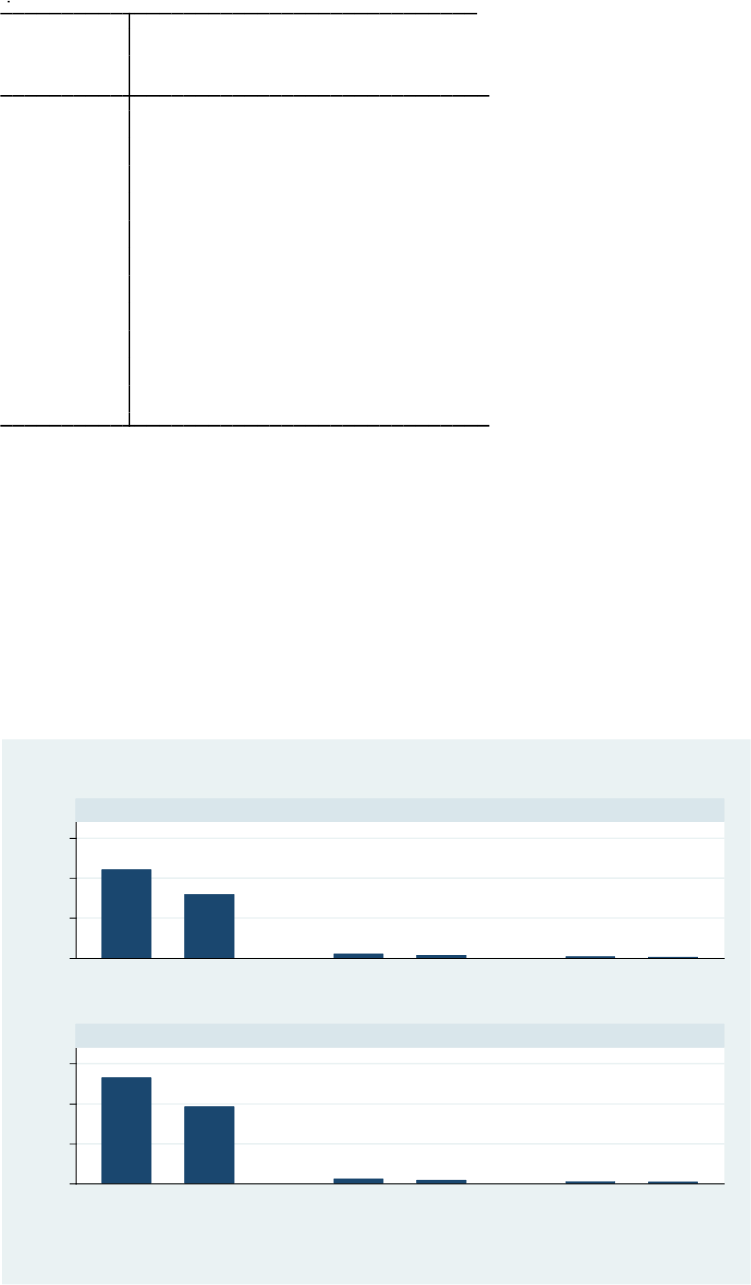
As another example, we can produce a meaningful graph quickly. We look at infant death rates in
Chile in this example.
. hmddata use lifetables , grid(5x10) popfilter(chile) clear
. hmddata intervals
. graph bar (asis) mx if inlist(age, 0, 1, 5) & inlist(sex, 1, 2) ,
over(yearstr) over(agestr) by(sex, col(1) title(Infant Death
Rates in Chile)) nofill
hmddata intervals generated a variable that enabled us to label the age categories nicely.
0.0215 0.0239 0.0258
60-64 0.0078 0.0092 0.0080
0.0073 0.0045 0.0049
20-24 0.0005 0.0007 0.0005
0.0104 0.0207 0.0115
1-4 0.0002 0.0003 0.0002
0.1027 0.1335 0.1079
0 0.0038 0.0041 0.0037
interval Italy Portugal Spain
Age Country / Population name
0
.005
.01
.015
0
.005
.01
.015
0 1-4 5-9
0 1-4 5-9
1992-1999 2000-2005 1992-1999 2000-2005 1992-1999 2000-2005
1992-1999 2000-2005 1992-1999 2000-2005 1992-1999 2000-2005
female
male
Central death rate at age x
Graphs by Sex
Infant Death Rates in Chile

8
As a second graph example, we create a scatter plot of life expectancy versus the infant mortality
rate for all HMD countries. We apply different marker colors for each half-century in order to
visualize the development over time.
. hmddata use lifetables bothsexes , grid(5x10) clear
. keep if mod(year,10)==0 & yearinterval==10 & age==0
A few auxiliary statements are necessary for the coloring of the marker variable:
. gen y50 = int((year-1700) / 50)
. label define Y50 1 "1750-" 2 "1800-" 3 "1850-" 4 "1900-" 5 "1950-"
6 "2000-"
. label values y50 Y50
. decode y50 , gen(y50_str)
. bys y50 age : replace y50_str = "" if _n!=1
. local scopts mlab(y50_str) mlabpos(2) mlabgap(*30) mlabsize(huge)
ylab(30(10)90) xlab(0(0.05)0.4)
The graph statement is:
7
. graph twoway ///
(sc ex mx if y50==1 & age==0, mstyle(p1) `scopts') || ///
(sc ex mx if y50==2 & age==0, mstyle(p2) `scopts') || ///
(sc ex mx if y50==3 & age==0, mstyle(p3) `scopts') || ///
(sc ex mx if y50==4 & age==0, mstyle(p4) `scopts') || ///
(sc ex mx if y50==5 & age==0, mstyle(p5) `scopts') || ///
(sc ex mx if y50==6 & age==0, mstyle(p6) `scopts') , ///
title("Life Expectancy at Birth and Infant Mortality Rates, All
HMD Countries", size(medium)) legend(off)
7
You may have noticed that the resulting graph has an inaccurate X-axis title: It says "Central death rate at age
x", while the graph depicts death rates at age 0. This is because the variable mx in the data set retrieved by
hmddata use really does contain death rates at all ages ("at age x"). In the example we deleted all ages
except 0, so the variable now only contains rates at age 0, but hmddata has no way of knowing this, so it does
not delete the variable label of mx which is used in the graph. This underscores that hmddata can be used to
quickly generate nicely labeled tables and graphs, but that the labeling may not always be perfect. In these
cases you may wish to further supply labeling information; here, using the xtitle() option. Analogous
comments for the Y-axis title in the example graph apply.

9
Up to now we have looked at graphs generated by standard Stata graph commands. We now explore
the graph subcommand of hmddata, which facilitates the quick generation of graphs that are a bit
more involved.
In the following, we use data from East and West Germany:
. hmddata use lifetables , grid(5x10) clear
. keep if yearinterval==10
. hmddata popfilter germanyeast germanywest, dummy(ger)
. hmddata intervals
hmddata graph provides a flexible syntax to specify dimensions and levels along which line
graphs shall be generated. We look at the development of infant mortality and life expectancy over
time again.
. hmddata graph line ex year if ger , at1(age 0 1) at2(sex female
male) by(pop)
65.0 70.0
75.0
80.0
1960 1970 1980 1990 20001960 1970 1980 1990 2000
Germany: East Germany Germany: West Germany
age==0 & sex==female age==0 & sex==male
age==1 & sex==female age==1 & sex==male
Remaining life expectancy at age x
Year
Graphs by Country / Population name

10
If we want to present the same information by sex instead of by region, we just have to juggle option
arguments a little:
. hmddata graph line ex year if ger & sex!=3 , at1(age 0 1) at2(pop)
by(sex, leg(col(1))) leg(size(vsmall))
Conclusion
This technical report introduced a Stata add-on module called "hmddata". It facilitates importing and
working with data from the Human Mortality Database (HMD). Both usage of HMD data and of the
hmddata tool are free of charge, and data access and installation are quick and easy. Many more
details and additional topics related to hmddata, such as data updates and replicability, are discussed
in the Stata help files that come with the package.
Acknowledgements
I thank Dmitri Jdanov, Tim Riffe, Vladimir Shkolnikov, and the staff of the Demographic Data Lab of
the Max Planck Institute for Demographic Research for helpful comments.
65.0 70.0
75.0
80.0
1960 1970 1980 1990 20001960 1970 1980 1990 2000
female male
age==0 & popname==Germany: East Germany age==0 & popname==Germany: West Germany
age==1 & popname==Germany: East Germany age==1 & popname==Germany: West Germany
Remaining life expectancy at age x
Year
Graphs by Sex

11
References
Human Mortality Database. University of California, Berkeley (USA) and Max Planck Institute for
Demographic Research (Germany). Available at www.mortality.org and
www.humanmortality.de.
Hyndman, Rob J. (2017): demography: Forecasting Mortality, Fertility, Migration and Population
Data. R package version 1.20.
Minton, Jon (2015): Merging, Exploring, and Batch Processing Data from the Human Fertility
Database and Human Mortality Database. Technical Report TR-2015-001, Max Planck Institute
for Demographic Research (MPIDR). URL
http://www.demogr.mpg.de/papers/technicalreports/tr-2015-001.pdf.
Riffe, Tim (2015): Reading Human Fertility Database and Human Mortality Database Data into R. .
Technical Report TR-2015-004, Max Planck Institute for Demographic Research (MPIDR). URL
http://www.demogr.mpg.de/papers/technicalreports/tr-2015-004.pdf.
Shkolnikov, Vladimir M. and Dmitri A. Jdanov (2016): R Programs for Writing HMD Life Tables and
HMD Death Rates to Pooled Data Files. Technical Report 2016-001, Max Planck Institute for
Demographic Research (MPIDR). URL http://www.demogr.mpg.de/papers/technicalreports/tr-
2016-001.pdf.
