
SMU Data Science Review SMU Data Science Review
Volume 2 Number 3 Article 12
2019
Quantitative Model for Setting Manufacturer's Suggested Retail Quantitative Model for Setting Manufacturer's Suggested Retail
Price Price
Peter Byrd
Southern Methodist University
Jonathan Knowles
Southern Methodist University
Dmitry Andreev
Southern Methodist University
Jacob Turner
Southern Methodist University
Brian Mente
KidKraft
See next page for additional authors
Follow this and additional works at: https://scholar.smu.edu/datasciencereview
Part of the Applied Statistics Commons, Multivariate Analysis Commons, Sales and Merchandising
Commons, and the Statistical Models Commons
Recommended Citation Recommended Citation
Byrd, Peter; Knowles, Jonathan; Andreev, Dmitry; Turner, Jacob; Mente, Brian; and Wallace, LaRoux (2019)
"Quantitative Model for Setting Manufacturer's Suggested Retail Price,"
SMU Data Science Review
: Vol. 2:
No. 3, Article 12.
Available at: https://scholar.smu.edu/datasciencereview/vol2/iss3/12
This Article is brought to you for free and open access by SMU Scholar. It has been accepted for inclusion in SMU
Data Science Review by an authorized administrator of SMU Scholar. For more information, please visit
http://digitalrepository.smu.edu.

Quantitative Model for Setting Manufacturer's Suggested Retail Price Quantitative Model for Setting Manufacturer's Suggested Retail Price
Authors Authors
Peter Byrd, Jonathan Knowles, Dmitry Andreev, Jacob Turner, Brian Mente, and LaRoux Wallace
This article is available in SMU Data Science Review: https://scholar.smu.edu/datasciencereview/vol2/iss3/12
Quantitative Model for Setting Manufacturer’s
Suggested Retail Price
Dmitry Andreev
1
, Peter Byrd
1
, Jonathan Knowles
1
, Dr. Jacob Turner
1
, Brian
Mente
2
, and LaRoux Wallace
2
1
Master of Science in Data Science, Southern Methodist University, Dallas TX
75275 USA {dandreev,peterb,jknowles,jturner}@smu.edu
2
KidKraft, 4630 Olin Road, Dallas, TX, 75244, United States {brian.mente,
laroux.wallace}@kidkraft.com
http://www.kidkraft.com/
Abstract. In this paper, we present a quantitative approach to model
the manufacturer’s suggested retail price (MSRP) for children’s doll-
houses and establish relationships among key features that contribute
most to establishing MSRP. Determination of the MSRP is a critical
step in how consumers respond with their wallets when purchasing an
item. KidKraft, a global leader in toys and juvenile products, sets MSRP
subjectively using product experts. The process is arduous and time con-
suming requiring the focus of specialized resources and knowledge of the
interaction between key attributes and their impact on consumer value.
An accurate prediction of MSRP during the early stages of the design
process is critical to aligning the cost of design features with the expected
revenue. Finding out that the MSRP is set incorrectly too late in the de-
sign process can result in costly redesign. Four models are constructed
for a simple objective approach to calculating a dollhouses MSRP. Each
model is evaluated for accuracy and simplicity, and a model using lin-
ear regression with forward selection is chosen based on ease of inter-
pretation, limited sample size and to prevent over-fitting. The top five
features with the greatest impact on MSRP are also highlighted. The
chosen model allows for a quick and easy determination of MSRP and
can validate that proposed features align with the predicted MSRP while
still early in the design process.
Keywords: KidKraft · Manufacturer’s Suggested Retail Price · MSRP
1 Introduction
Setting the right price for goods and services is an age-old problem in the retail
world. With the explosive growth of online shopping within the last decade[1],
companies are reevaluating their pricing strategies. Before rushing into a price
matching war with their competitors, an objective must be defined. Retailers
confront a seemingly impossible dual competitive challenge: grow the top line
revenue while also preserving their bottom line. Innovations in pricing and pro-
motion provide considerable opportunities to target customers effectively both
1
Byrd et al.: Quantitative Model for Setting MSRP
Published by SMU Scholar, 2019
offline and online[5]. Different pricing practices are emerging that refer to the
use of information on customer value, competition, and costs respectively[6].
Some companies are looking to maximize profits on each unit sold, while oth-
ers are trying to protect a certain share of their market. To keep up with the
ever-changing behaviors of the typical consumer, retailers are moving away from
relying heavily on traditional methods for setting the manufacturer’s suggested
retail price in favor of using data-driven techniques for faster and more accurate
pricing[4].
Determining MSRP is difficult and time consuming and requires significant
product expertise[7]. Design inputs such as construction, materials, accessories,
number of levels, competition, and many others each contribute to the real and
perceived value of a product. Each influence, at different levels, the final MSRP
for the product. Currently, new product pricing requires product experts in each
product category to leverage their experience along with product features and
publicly available competitive information to determine an appropriate MSRP.
This puts a heavy emphasis on knowledgeable product experts and increases the
potential for human error.
Finding that the MSRP is set incorrectly late in the design process can be
very expensive. Expected revenues from product sales must align with the costs
associated with certain features to ensure acceptable margins for the business.
Uncovering an MSRP misaligned with cost late in the design process may re-
quire redesign and exclusion of some of the features in the original design plan.
Calculating the MSRP early in the design process can save money by limiting
product redesign.
We create an automated model to determine the MSRP given the product
features and categories. This offers a quick and easy way to align expected rev-
enue with key features and provides the flexibility to adjust design plans before
construction begins. We also make the connection between key features and the
impact each has on the MSRP for the product.
KidKraft provided a list of five-hundred products they manufacture. There
are six distinct categories: dollhouses, roll play, toddler toys, vehicle play-sets,
furniture, and outdoor. Each item is described with its dimensions and a long list
of features that make it unique. Publicly available information on competitors
was also included. Product features are reorganized into discrete values and used
as the basis for price modelling.
The data consists of a relatively small number of rows, with a large number
of features for each item. One-hot encoding was used on categorical and ordinal
features to prepare them for use in the regression models. The amount of data
available by product category doesn’t lend itself to deep learning algorithms
or similar advanced learning techniques and falls into the realm of traditional
statistics.
Several highly correlated features were present during exploratory data anal-
ysis, and feature reduction was required to close in on a stable model. Ridge,
Lasso and Elastic Net regression are equipped to handle highly correlated fea-
tures and therefore were also used in the model evaluations. For the general linear
2
SMU Data Science Review, Vol. 2 [2019], No. 3, Art. 12
https://scholar.smu.edu/datasciencereview/vol2/iss3/12
model, a feature reduction of highly correlated features included the removal of
height, width, length, competitor indicator, product number, and material. All
four regression models produced accurate results with limited errors. The de-
pendent variable was defined as MSRP, and within each category the product
features are the independent variables.
The chosen solution was a general linear model with forward selection. Pre-
diction errors were limited, and good model interpretation was a key factor in
the selection. A limited number of MSRP values per product required forward
selection of parameters to identify the features with the greatest impact to deter-
mining MSRP and prevent a long list of features with small incremental impact.
Based on the linear model with forward selection, the top five features impacting
MSRP are: x8, x7, x10, x9, and x14.
Another interesting observation from the model is the impact of the value
attribute x9 has on MSRP. Predicted MSRP has a positive relationship with
this attribute. However, there does appear to be a point of diminishing returns.
Additionally, inclusion of attribute x14 to a dollhouse design appears to have a
strong positive affect, increasing the MSRP when this attribute is included.
Model performance shows good residual distribution across the MSRP price
range, and the Normal Q-Q plot verifies our assumption of a normal distribution
of MSRP values. BIC optimization shows the best performance with five model
predictors without over-fitting the data. Mean squared error of predicted MSRP
vs. actual MSRP is strong for all models with ranges from 1028 to 1830.
A linear regression model with forward selection provides a means for quickly
determining the MSRP for dollhouses based on key product features. Leveraging
this simple model in the early stages of the design process for building children’s
toys can ensure that design features align with the expected revenue. As a valida-
tion tool for product experts, the model is capable of catching errors in MSRP
calculations and avoiding costly design changes. By leveraging advanced sta-
tistical techniques, this research provides an approach for KidKraft to set and
validate the MSRPs in conjunction with their product experts.
2 Related Work
Few published articles detail approaches to set the manufacturer’s suggested
retail price. Most are focused on value delivery versus cost of production. The
study of Successful New Product Pricing Practices delves into the conditions
upon which success is contingent and ”distinguishes three different pricing prac-
tices that refer to the use of information on customer value, competition, and
costs respectively[6].” Although the focus of this research is similar to our objec-
tive of setting product prices, the framework described centers more on pricing
strategy than an automated tool to determine MSRP.
In an article from The McKinsey Quarterly, using value to determine price is
explored. ”The trade-off between benefits and price has long been recognized as
3
Byrd et al.: Quantitative Model for Setting MSRP
Published by SMU Scholar, 2019

a critical marketing mix component[1].”
1
The article emphasizes the importance
of setting price based on consumer value and not on cost alone. The approach
we use takes this further with the creation of an automated model that leverages
feature value for price setting. Our evaluation of products features determines
how valuable a specific feature is and feeds into the model for determining price.
When creating a prediction model, a good practice to follow is starting with
the simplest model for the task at hand as Ameisen points out in his Medium blog
post[2]. Using a simple model as a baseline can provide a better understanding
of the dataset such as feature importance and what direction to take in terms of
refining the model. After establishing the baseline, more complex models such
as elastic net are explored[15]. This is somewhat generic guidance, but good
practice. We follow this approach using a baseline linear regression model as a
first step in analysis prior to model optimization.
In Selim’s Determinants of house prices in Turkey: Hedonic regression versus
artificial neural network, home values are determined using “multiple regression
techniques on large data sets[11].” The use of regression techniques for deter-
mining house values is very similar to the approach being used for calculating
the price of toys. We can draw similarities between Selim’s approach and our
problem of determining the price of a dollhouse. However, data on house prices
is significantly larger which allows for advanced techniques like deep learning.
These techniques will not work on our much smaller set of product information
and the approach must be adapted without the use of deep learning algorithms.
In Smith’s Clearance pricing and inventory policies for retail chains, a cal-
culation of clearance pricing is performed based on “price, seasonal effects, and
the remaining assortment of items available to customers[12].” This is another
example of leveraging key attributes to determine optimal pricing. Smith also
points out a similar concern that “pricing errors result in either loss of potential
revenue or excess inventory[12].” Although the approach is similar, the objective
is different. Our focus is on setting a price based on key attributes, whereas
Smith is modifying price to limit inventory and maximize revenue.
3 KidKraft
KidKraft is an industry-leading global business. Their toys are sold in more than
90 countries by more than 28,000 sellers worldwide. KidKraft is well-known for
their award-winning dollhouses and play kitchens, and have expanded product
categories to also include train-sets, play-sets, furniture, swing-sets, playhouses,
and the World of Eric Carle. KidKraft is focusing efforts on quantifying the
relationship between descriptive features of products within a given category
of toys and the MSRP for those toys. Inputs such as construction, materials,
accessories, number of levels, competition, and many others each contribute to
1
More information may be found at https://www.mckinsey.com/business-
functions/marketing-and-sales/our-insights/setting-value-not-price. Last accessed 5
Jun 2019.
4
SMU Data Science Review, Vol. 2 [2019], No. 3, Art. 12
https://scholar.smu.edu/datasciencereview/vol2/iss3/12
the real and perceived value of a product and each influence, at different levels,
the final MSRP for the product.
KidKraft is best known for their dollhouses. They come in many different
sizes and categories including platforms for 5 inch, 12 inch and 18 inch dolls. As
the largest product category in their range of children’s toys, this is our primary
focus for predicting MSRPs.
3.1 KidKraft Method for Determining MSRP
At KidKraft, manufacturer’s suggested retail price is currently set by product
experts that spend years achieving the experience required to determine the
retail price of a new product. This requires intimate knowledge of each feature
that is part of the product, as well as a clear picture of the customer value
for those features. Not only is it critical for the product expert to understand
feature values for the new product, but it is also important that they know what
competitors are introducing to the market and how it compares to the feature
set of the new product. The pricing strategy includes a decision on pricing on
value, competition, or cost, and likely includes some combination to set the final
price.
Pricing for new products consists of a combination of toy category, features,
competitor comparison, and current market dynamics. Product experts gain an
understanding of what features contribute the most value to a new product,
and through competitive analysis can begin to make decisions on setting a price
point.
This level of knowledge is not easily obtained and requires years of invest-
ment in human capital to efficiently set the MSRP for new products in each toy
category. Human error is a concern and mistakes can be very costly. Improp-
erly setting the initial price of a product has ramifications to consumer demand,
product market share, product margins and company profitability.
4 Exploring Product Categories
The five-hundred items in the KidKraft product lineup provided are grouped
into six major categories: Dollhouses, Roll Play, Toddler Toys, Vehicle Playsets,
Furniture and Outdoor. Each major category is further segmented into sub-
categories. There are a total of 52 sub-categories. The sub-categories are an
independent variable used in modeling, and models are grouped by the six major
categories.
Based on the available data within each category, a decision was made to
narrow the focus to a group of categories with a high amount of records. The
product categories used in modeling include: Dollhouses for 5’ dolls, Dollhouses
for 12” dolls, Dollhouses for 18” dolls, and Mansion Dollhouses for 12” dolls. A
further description of dollhouse variables is included later in this document.
5
Byrd et al.: Quantitative Model for Setting MSRP
Published by SMU Scholar, 2019
5 Tutorial Topics
Our approach to predicting MSRP based on product details compares multiple
models to determine which provides the best performance. A small data set with
limited items and many features doesn’t have a sufficient number of records for
deep learning techniques and requires a traditional statistics approach. GLM,
Ridge regression, Lasso regression, and Elastic Net are all considered. More
information of each of these model approaches is included in this section.
5.1 General Linear Model
The general linear model (GLM) is a statistical method which is used to relate
responses to the linear sequences of predictor variables, such as dimensions and
features. In our case, the dependent response variable is manufacturers suggested
retail price, and the predictor variables are dimensions, features, categories, and
many more. GLM is widely used in applied research.
GLM is the basic method for the Analysis of Variance (ANOVA), Analysis
of Covariance (ANCOVA), t-test, f-test, regression analysis, and most of the
multivariate techniques like canonical correlation, cluster analysis, discriminant
function analysis, factor analysis, multidimensional scaling, and many more[9].
The general linear model is a useful framework determining how a set of
independent variables affect a continuous variable. The base formula for a general
linear model takes the form:
ˆ
Y = β
0
+ β
1
X (1)
In the equation above,
ˆ
Y is the dependent response variable, in our case
MSRP. β
0
is the intercept of the equation. β
1
is a coefficient which determines
how much each variable contributes, and X is a predictor variable such as height,
weight, material, etc.
This procedure isn’t restricted to only a single variable but can handle a wide
variety of variables, including a non-numerical ones. These categorical variables
are encoded to numeric variables for regression analysis. Some manipulation of
the product features are required to create discrete variables. The expanded
regression formula takes the form:
ˆ
Y = β
0
+ β
1
X
1
+ β
2
X
2
...β
n
X
n
(2)
Regression is a univariate general linear model. Univariate GLM is a method
which is used in Analysis of Variance for experiments having two or more factors.
GLM ANOVA analysis for determining an MSRP in this setting is performed
using a number of steps which are described in Table 1 below.
Step 1: Check variables After initial data cleaning, the continuous and cate-
gorical variables are separated. The distribution of the continuous variables are
checked and scaling issues taken care of. A check for outliers is also performed to
determine if they are present and how to handle them. Categorical variables may
6
SMU Data Science Review, Vol. 2 [2019], No. 3, Art. 12
https://scholar.smu.edu/datasciencereview/vol2/iss3/12

Table 1. GLM Analysis Steps
Process Steps Brief Description of Steps
Step 1 Check variables
Step 2 Feature engineering
Step 3 Summary statistics
Step 4 Train and test set
Step 5 Build the model
Step 6 Assess performance
Step 7 Improve the model
require encoding to numeric values, and plots of the distribution of the response
variable for each category is useful.
Step 2: Feature engineering Some of the features may need to be recast to
be statistically meaningful. Others may have no impact on the result and may
be considered for omission.
Step 3: Summary statistics A set of summary statistics should be created to
validate assumptions are met. Interactions between variables should be evalu-
ated, and a visualization of the correlation between variables produced. Highly
correlated predictor variables may require other techniques such as Ridge, Lasso,
or Elastic Net regression.
Step 4: Train and test set Data should be split between training and test sets
for model evaluation. Model parameters will be determined using the training
data, and accuracy checked by predicting the response for the test set.
Step 5: Build the model Once the data is prepared, select the appropriate
response and independent predictor variables and set the model to run. Results
should include a plot of means with confidence intervals, typically set for alpha
equal to 0.05, with p-values for each variable to show their significance.
Step 6: Assess performance Performance of the model can be measured using
metrics such as AIC, BIC, adjusted R squared or mean squared error (MSE).
Assumptions of normality and equal variance should be verified as part of the
analysis.
Step 7: Improve the model Identify which effects and interactions are sig-
nificant by reviewing the p-values for each predictor. Further simplification of
the model may be possible by removing highly correlated predictors via Ridge,
Lasso or Elastic Net. This may also lead to a model that is easier to interpret.
The ordinary least squares estimator is unbiased, however, it can have a large
variance especially when the predictor variables are highly correlated or there
are a large number of predictors relative to the size of the data set. This can
result in an unreliable model.
To counter this we may elect to reduce variance at the cost of introducing
some bias. This approach is called regularization and is almost always beneficial
for the predictive performance of the model. There are three popular techniques
for achieving this: Ridge Regression, Lasso Regression, and Elastic Net.
7
Byrd et al.: Quantitative Model for Setting MSRP
Published by SMU Scholar, 2019
5.2 Ridge Regression
Ridge regression is a technique used to analyze data which is multicollinearity
in nature. It is a remedial measure taken to alleviate multicollinearity amongst
regression predictor variables in a model. This occurs when there are high cor-
relations between multiple predictor variables.
Often predictor variables used in a regression are highly correlated. When
they are, the regression coefficient of any one variable depends on the other
predictor variables included in the model. The predictor variable does not reflect
any inherent effect on the response variable, but only a marginal effect, given the
other correlated predictor variables being used. Ridge regression adds a small
bias factor to the variables in order to alleviate this problem.
Ridge regression addresses the issue of multicollinearity by shrinking the co-
efficient estimates of the highly correlated variables, and in some cases shrinking
it close to zero thus effectively removing the influence of the variable.
Ridge regression performs L2 regularization. A penalty is calculated by mul-
tiplying the tuning parameter, λ, by the square of the magnitude of coefficients.
When λ = 0, it is similar to least squares regression. When λ is large, the sen-
sitivity of the response to the predictor variable is minimized. Ridge regression
doesn’t result in the elimination of coefficients, and therefore doesn’t result in
sparse models.
5.3 Lasso
Lasso regression is another type of linear regression that encourages simple,
sparse models, by using shrinkage to reduce the number of predictor parameters.
It is used for variable selection and parameter elimination to simplify models and
make them easier to interpret. Similar to ridge regression, lasso regression is will-
suited for models with high levels of multicollinearity. The acronym “LASSO”
stands for Least Absolute Shrinkage and Selection Operator. Lasso regression
differs from Ridge regression is that it can effectively eliminate variables used in
the model as opposed to only minimizing their affect on the response.
Whereas Ridge regression uses L2 regularization, Lasso regression performs
L1 regularization, which adds a penalty equal to the absolute value of the mag-
nitude of coefficients. Some coefficients can become zero and eliminated from the
model all together. This is ideal for producing simpler models and makes Lasso
far easier to interpret and prevents over-fitting.
A tuning parameter, λ controls the strength of the L1 penalty. When λ =
0, no parameters are eliminated and the estimate is equal to the one found
with linear regression. The higher you set λ the more penalty is applied to the
coefficients and the smaller the coefficients will be with some potentially going
to zero.
5.4 Elastic Net
Elastic Net combines the penalties of ridge and lasso regression. It incorporates
penalties from both L1 and L2 regularization. In addition to choosing a lambda
8
SMU Data Science Review, Vol. 2 [2019], No. 3, Art. 12
https://scholar.smu.edu/datasciencereview/vol2/iss3/12

value, elastic net also uses an alpha parameter where α = 0 corresponds to ridge
and α = 1 to lasso, and we can optimize the model by adjusting alpha between
0 and 1.
6 Data Set
The data set we use in our analysis contains 85 records of dollhouses with 21
variables captured for each. To describe the variables we have broken the vari-
ables down by whether they are continuous or categorical and provided a brief
description and examples values for each.
Table 2. Continuous Variables
Continuous Variable Example Value(s)
MSRP 119.99
x3 47.5
x4 13.25
x5 34.25
x6 22763.92
x7 28.6
x9 3
x10 11
x15 2
x16 21
Table 3. Categorical Variables
Categorical Variable Example Value(s)
x1 945867
x2 Yes, No
x8 5, 12, 18
x11 Yes, No
x12 Yes, No
x13 Yes, No
x14 Yes, No
x17 1, 2, 3, 4
x18 Yes, No
x19 Yes, No
x20 Yes, No
x21 Yes, No
Because we are working with a smaller data set, only 85 records, we will be
restricted in the types of regression methods we can perform, and we discus this
9
Byrd et al.: Quantitative Model for Setting MSRP
Published by SMU Scholar, 2019
later in this paper. With a large number of relevant potential predictor variables,
20, we have potential to understand which specific features have the most impact,
if any, when determining what the MSRP of a dollhouse should be; and as the
features and their values are descriptive it will ease in the interpretation of the
model we produced.
7 Exploratory Data Analysis
To gain insight into the categorical variables, we created a barplot of each vari-
able against MSRP. The data seems to meet the assumptions for regression and
there was nothing that would indicate a transformation being required for any
of the variables. In reviewing the plots, a single outlier was identified that was
expanding the scale of our diagrams; when we reviewed our findings with a sub-
ject matter expert from KidKraft they informed us that this record was indeed
an outlier and should be removed. Figures 1 and 2 show that we do not see
any issues with distribution, the means, or standard deviations that will cause
any issues with our regression analysis.
Continuous variables in the dataset are examined to check for relationships
between explanatory variables and the target variable. To compare the relation-
ship of each continuous variable against MSRP and the distribution between
them we created the table of paired scatterplots with their distributions included
in Figure 3. In examining the table we are looking for polynomial or non-linear
relationships between our potential explanatory variables and our target vari-
able, as well as uneven or a skewed distribution of the values. As Figure 3 shows,
there are no issues regarding non-linear relationships or uneven distribution of
the values in the dataset.
8 Model Selection and Predictions
When approaching a prediction task for a continuous variable, it is good practice
to create a baseline model[2]. Without knowing how each predictor variable
affects the MSRP of toys, applying a general linear model is a logical starting
point. In this scenario, the model suggests that the MSRP increases on a linear
scale as the size of the toys increase and they include more features. However,
this could place too much emphasis on a few of the most important predictor
variables while essentially ignoring the remaining majority of predictors. Due to
the simplicity of such a model, predictions may be less accurate than that of
alternative models.
The next step to explore is the possibility of non-linear behavior of MSRP.
The dataset has high dimensionality so without prior knowledge of which predic-
tor variables have the highest importance with relation to MSRP, it doesn’t seem
reasonable to discard of any of them. Rather than implementing every regres-
sion algorithm available for the sake of improved accuracy, the ridge regression
model proved to be a suitable next step. The dataset also has several variables
that are highly correlated which can ultimately affect the prediction accuracy of
10
SMU Data Science Review, Vol. 2 [2019], No. 3, Art. 12
https://scholar.smu.edu/datasciencereview/vol2/iss3/12

Fig. 1. Barplots for EDA of categorical variables
the model if not properly accounted for. Despite having gone through the pro-
cess of feature reduction, ridge regression helped to further reduce any effects of
multicollinearity from the variables that we kept after EDA.
Since the ridge regression method aims to keep all the available variables, we
noticed that the majority of them had almost negligible estimators and decided
to try the Lasso regression method. In doing so, the number of predictor variables
used dropped significantly from 20 down to 6. This makes for a less complex
model that is easier to interpret and explain how each feature impacts the MSRP
to the end user at KidKraft.
As a middle ground between ridge and lasso regression, we wanted to see how
elastic net would compare. Using this method, we keep 15 predictor variables
which falls between the number used in the lasso and ridge models. Once again,
we see that the majority of these variables have negligible coefficients and only
6 out of the total of 15 had a coefficient large enough to suggest an actual
relationship with MSRP.
11
Byrd et al.: Quantitative Model for Setting MSRP
Published by SMU Scholar, 2019

Fig. 2. Barplots for EDA of categorical variables
Since we did see a reduction in the model MSE of 1830 for ridge regression
down to 1115 for lasso regression and an even further reduction down to 1028
when applying elastic net, we felt that we were moving in the right direction by
using a feature selection algorithm. With this in mind and the desire to have a
model that can be easily explained, we reverted back to the initial GLM to see
if we could add a feature selection method. To meet the aforementioned require-
ments, we found that a forward selection method provided us with an optimal
solution. By using the BIC metric as our stopping criteria, the model required
only five predictor variables to give an accurate prediction which included the
features: x8, x7, x10, x16, and x14.
9 Performance and Results
After selecting GLM with forward selection method as our final model, we pro-
ceeded to look at the standard statistical diagnostic plots to ensure the assump-
12
SMU Data Science Review, Vol. 2 [2019], No. 3, Art. 12
https://scholar.smu.edu/datasciencereview/vol2/iss3/12

Fig. 3. Pairplot to check for normal distribution and evidence of correlation amongst
continuous variables
tions for a linear model have been met. Throughout this section, we will be
referring to the Figure 4 on the next page.
To start, the normality assumption is satisfied since the Q-Q plot of residuals
follows a straight line trend[3]. There is a slight downward deviation at the top
right corner of the plot suggesting that the model is slightly skewed at the higher
end of MSRP. A majority of the dollhouses that we encountered during EDA
fell within the $50 - $300 price range, however, there were several limited edition
items that were above $500. Since there are a limited number of products that
are priced that high, it is logical that the model encounters larger errors when
trying to predict their MSRP. Considering the skewness is slight and the lack of
data points at the higher price range, we felt that the overall straight line trend
for the normality assumption was reasonable[14].
For the equal standard deviation assumption, the residuals plot didn’t pro-
vide any strong evidence for a change along the entire price range. For this
reason, we consider this assumption to be met. When looking at the Cook’s
13
Byrd et al.: Quantitative Model for Setting MSRP
Published by SMU Scholar, 2019
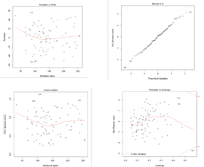
Fig. 4. Diagnostic plots to check model assumptions for GLM with forward selection
distance plot, we did not encounter any highly influential data points[10] which
makes sense because any extreme or missing values had already been dealt with
during EDA. Lastly, the independence assumption is also met[8] as we reduced
any variables that showed high correlations, such as the dollhouse length, width,
and height. These variables were combined into a single volume variable which
is depicted in the evenly distributed residuals plot.
10 Ethics
There is an increasing focus on ethics surrounding even the most common busi-
ness practices. Determining the manufacturer’s suggested retail price for chil-
dren’s toys is no exception to this emphasis. Establishing an objective approach
based on the presence of key features and competition, provides a foundation
for an ethical approach to price setting. The method presented provides for
consistent and fair product pricing across the entire business, regardless of the
employee responsible for pricing or the customer purchasing the product. The
result is an efficient and consistent one for the employee making it easier to
14
SMU Data Science Review, Vol. 2 [2019], No. 3, Art. 12
https://scholar.smu.edu/datasciencereview/vol2/iss3/12
perform their job without error and establish MSRP estimates based on past
results.
There is a responsibility to understand and communicate the boundaries and
limits of the regression approach to modeling prices. Misrepresentation of the
capabilities of the model as a end all solution should be avoided. While the model
can be an effective tool for determining and validating manufacturers suggested
retail price, it is likely not a replacement for employing product experts. The
value a product expert provides goes beyond the bounded inputs used in the
model. Representation of the model as an alternative to the vast experience and
capabilities of product experts is a misrepresentation of the model that over
emphasizes its capabilities and diminishes the breadth and depth of experience
of the experts. A cost benefits analysis should not assume the value of the model
to be equivalent to the operating expense of employing and maintaining product
experts.
For the consumer, the process ensures that they are treated fairly despite the
individual product expert, market fluctuations, or seasonal influences, and that
they are protected against even unintentional inconsistencies in pricing. This can
prevent price manipulation at busy times of the year and ensure the delivery of
a clear and consistent price for all high-end children’s toys.
Another consideration is security and privacy of the model. The model is
purpose built based on pricing strategies at KidKraft. Extending the specific
model to competitors is a violation of a non-disclosure agreement and reveals
internal pricing practices. Leaking this information may provide competitors
with an unfair pricing advantage and negatively impact product sales. Like all
internal intellectual capital, this model should be protected with the same level
of rigor as all other company data. Sharing the model algorithm, with or without
the data used to create it, is an unethical act, and potentially criminal.
In providing this model to the company, we offer a data driven approach free
of human motives that could influence product pricing. An objective model is
built to ensure the most accurate MSRP based on consumer value that specific
features provide. As developers of the pricing model, responsibility rests on us
to make certain we offer an objective model that supports business objectives
and aligns with consumer value.
11 Conclusion
Accurate, objective, data driven prediction of MSRP based on product category
and key product features is a valuable tool that can be used by product ex-
perts to determine a product’s initial starting price[13]. This saves time during
pricing and validates design features before construction. Using this quantita-
tive model as a tool during the design process, KidKraft can validate that the
proposed features for a new toy being developed align with the predicted MSRP
while still early in the design and phase. If the model predictions don’t agree
with the opinion of the product experts, KidKraft can take this opportunity
to understand what is driving this misalignment and quickly react to make the
15
Byrd et al.: Quantitative Model for Setting MSRP
Published by SMU Scholar, 2019
necessary changes before beginning the manufacturing process. Ultimately, this
will help minimize any mistakes in pricing that lead to costly redesigns and loss
of revenue.
References
1. Ali, F.: A decade in review: Ecommerce sales vs. retail sales 2007-2018. Dig-
ital Commerce 360 (Feb 2019), https://www.digitalcommerce360.com/article/e-
commerce-sales-retail-sales-ten-year-review/
2. Ameisen, E.: Always start with a stupid model, no exceptions.
https://blog.insightdatascience.com/always-start-with-a-stupid-model-no-
exceptions-3a22314b9aaa (3 2018), online, accessed on 2019-07-13
3. Augustin, Nicole H., E.A.S., Wood, S.N.: On quantile quantile plots for generalized
linear models. Computational Statistics Data Analysis 56(8), 2404–9 (August
2012), https://doi.org/10.1016/j.csda.2012.01.026
4. Bradlow, E., Gangwar, M., Kopalle, P., Voleti, S.: The role of big data and
predictive analytics in retailing. Journal of Retailing 93, 79–95 (03 2017).
https://doi.org/https://doi.org/10.1016/j.jretai.2016.12.004
5. Grewal, D., Ailawadi, K.L., Gauri, D., Hall, K., Kopalle, P., Robertson,
J.R.: Innovations in retail pricing and promotions. Journal of Retailing 87,
S43 – S52 (2011). https://doi.org/https://doi.org/10.1016/j.jretai.2011.04.008,
http://www.sciencedirect.com/science/article/pii/S0022435911000376, innova-
tions in Retailing
6. Ingenbleek, P., Debruyne, M., Frambach, R.T., Verhallen, T.M.M.: Successful
new product pricing practices: A contingency approach. Marketing Letters 14(4),
289–305 (Dec 2003). https://doi.org/10.1023/B:MARK.0000012473.92160.3d,
https://doi.org/10.1023/B:MARK.0000012473.92160.3d
7. Kienzler, M., Kowalkowski, C.: Pricing strategy: A review of 22 years of
marketing research. Journal of Business Research 78, 101–110 (05 2017).
https://doi.org/https://doi.org/10.1016/j.jbusres.2017.05.005
8. Osborne, J., Waters, E.: Four assumptions of multiple regression that researchers
should always test. Practical Assessment, Research Evaluation 8 (01 2002)
9. Ramsey, F., Schafer, D.: The Statistical Sleuth, A Course in Methods of Data
Analysis. Brooks/Cole, Cengage Learning, 20 Channel Center Street, Boston, MA
02210, 3 edn. (2013)
10. Sam Jayakumar, D., .A, S.: Exact distribution of cook’s distance and identifi-
cation of influential observations. Hacettepe University Bulletin of Natural Sci-
ences and Engineering Series B: Mathematics and Statistics 44, 165–178 (03 2015).
https://doi.org/10.15672/HJMS.201487459
11. Selim, H.: Determinants of house prices in turkey: Hedonic regression versus ar-
tificial neural network. Expert Systems with Applications 36, 2843–2852 (March
2009), https://doi.org/10.1016/j.eswa.2008.01.044
12. Smith, S.A., Achabal, D.D.: Clearance pricing and inventory policies
for retail chains. Management Science 44(3), 285–432 (March 1998),
https://doi.org/10.1287/mnsc.44.3.285
13. Subrahmanyan, S.: Using quantitative models for setting re-
tail prices. Journal of Product Brand Management 9 (2000).
https://doi.org/https://doi.org/10.1108/10610420010347100
16
SMU Data Science Review, Vol. 2 [2019], No. 3, Art. 12
https://scholar.smu.edu/datasciencereview/vol2/iss3/12
14. Theobald, C.M.: Generalizations of mean square error applied to ridge re-
gression. Journal of the Royal Statistical Society: Series B (Methodological)
36(1), 103–106 (September 1974). https://doi.org/https://doi.org/10.1111/j.2517-
6161.1974.tb00990.x
15. Zou, H., Hastie, T.: Regularization and variable selection via
the elastic net. Journal of the Royal Statistical Society 67,
301–320 (2005). https://doi.org/10.1111/j.1467-9868.2005.00503.x,
http://www.jstor.org/stable/3647580
17
Byrd et al.: Quantitative Model for Setting MSRP
Published by SMU Scholar, 2019
