
GLOBAL
EDITION
GLOBAL
EDITION
This is a special edition of an established title widely
used by colleges and universities throughout the world.
Pearson published this exclusive edition for the benefit
of students outside the United States and Canada. If you
purchased this book within the United States or Canada,
you should be aware that it has been imported without
the approval of the Publisher or Author.
Pearson Global Edition
Introduction to
Management Science
THIRTEENTH EDITION
Bernard W. Taylor III
THIRTEENTH
EDITION
Taylor
Using simple, straightforward examples to present complex mathematical concepts,
Introduction to Management Science builds a solid foundation in the logical application
of mathematical models and computing technology enabling students to make
decisions and solve problems. The hallmark features of this new and updated edition
include the following:
• Management Science Application boxes that aid in developing employability skills by
presenting modeling techniques and providing a framework for problem-solving.
• Over 800 homework problems and 69 cases that provide ample practice opportunities to
master the topics at hand.
• The Latest version of Excel
®
2016 with more than 175 spreadsheet screenshots that include
reference boxes to describe the solution steps.
• More than 60 new exhibit screenshots that present the latest versions of Microsoft
®
Project
2016, QM for Windows, Excel QM, TreePlan, and Crystal Ball.
• More than 550 updated Web links that provide access to tutorials, summaries, and notes
including links to YouTube videos.
Introduction to
Management Science
GLOBAL
EDITION
Taylor_13_1292263040_Final.indd 1 04/09/18 4:58 PM
Introduction to
Management Science
A01_TAYL3045_13_GE_FM.indd 1 29/10/2018 16:50
This page intentionally left blank
A01_PERL5624_08_GE_FM.indd 24 2/12/18 2:58 PM

Virginia Polytechnic Institute and State University
Harlow, England • London • New York • Boston • San Francisco • Toronto • Sydney • Dubai • Singapore • Hong Kong
Tokyo • Seoul • Taipei • New Delhi • Cape Town • Sao Paulo • Mexico City • Madrid • Amsterdam • Munich • Paris • Milan
13
th
Edition
Global Edition
Introduction to
Management
Science
Bernard W. Taylor III
A01_TAYL3045_13_GE_FM.indd 3 29/10/2018 16:50

Vice President, Business Publishing: Donna Battista
Director of Portfolio Management: Stephanie Wall
Director, Courseware Portfolio Management: Ashley Dodge
Senior Sponsoring Editor: Neeraj Bhalla
Editorial Assistant: Linda Albelli
Editor, Global Edition: Punita Kaur Mann
Associate Editor, Global Edition: Ananya Srivastava
Assistant Editor, Global Edition: Shasya Goel
Vice President, Product Marketing: Roxanne McCarley
Senior Product Marketer: Kaylee Claymore
Product Marketing Assistant: Marianela Silvestri
Manager of Field Marketing, Business Publishing: Adam Goldstein
Executive Field Marketing Manager: Thomas Hayward
Vice President, Production and Digital Studio, Arts and Business:
Etain O’Dea
Director of Production, Business: Jeff Holcomb
Managing Producer, Business: Melissa Feimer
Content Producer: Sugandh Juneja
Content Producer, Global Edition: Nitin Shankar
Manufacturing Controller, Global Edition: Caterina Pallegrino
Operations Specialist: Carol Melville
Design Lead: Kathryn Foot
Manager, Learning Tools: Brian Surette
Content Developer, Learning Tools: Lindsey Sloan
Managing Producer, Digital Studio and GLP, Media Production
and Development: Ashley Santora
Managing Producer, Digital Studio: Diane Lombardo
Digital Studio Producer: Regina DaSilva
Digital Studio Producer: Alana Coles
Digital Content Team Lead: Noel Lotz
Digital Content Project Lead: Courtney Kamauf
Project Managers: Roberta Sherman and Sree Meenakshi.R, SPi Global
Cover Designer: Lumina Datamatics, Inc.
Cover Art: Hluboki Dzianis / Shutterstock
Microsoft and/or its respective suppliers make no representations about the suitability of the information contained in the documents and related
graphics published as part of the services for any purpose. All such documents and related graphics are provided “as is” without warranty of any
kind. Microsoft and/or its respective suppliers hereby disclaim all warranties and conditions with regard to this information, including all warranties
and conditions of merchantability, whether express, implied or statutory, fitness for a particular purpose, title and non-infringement. In no event shall
Microsoft and/or its respective suppliers be liable for any special, indirect or consequential damages or any damages whatsoever resulting from loss of
use, data or profits, whether in an action of contract, negligence or other tortious action, arising out of or in connection with the use or performance of
information available from the services.
The documents and related graphics contained herein could include technical inaccuracies or typographical errors. Changes are periodically added
to the information herein. Microsoft and/or its respective suppliers may make improvements and/or changes in the product(s) and/or the program(s)
described herein at any time. Partial screen shots may be viewed in full within the software version specified.
Microsoft
®
and Windows
®
are registered trademarks of the Microsoft Corporation in the U.S.A. and other countries. This book is not sponsored or
endorsed by or affiliated with the Microsoft Corporation.
Pearson Education Limited
KAO Two
KAO Park
Harlow
CM17 9NA
United Kingdom
and Associated Companies throughout the world
Visit us on the World Wide Web at: www.pearsonglobaleditions.com
© Pearson Education Limited, 2019
The rights of Bernard W. Taylor III to be identified as the authors of this work have been asserted by them in accordance with the Copyright, Designs
and Patents Act 1988.
Authorized adaptation from the United States edition, entitled Introduction to Management Science, 13th Edition, ISBN 978-0-13-473066-0 by Bernard
W. Taylor, published by Pearson Education © 2018.
All rights reserved. No part of this publication may be reproduced, stored in a retrieval system, or transmitted in any form or by any means, electronic,
mechanical, photocopying, recording or otherwise, without either the prior written permission of the publisher or a license permitting restricted copying
in the United Kingdom issued by the Copyright Licensing Agency Ltd, Saffron House, 6–10 Kirby Street, London EC1N 8TS.
All trademarks used herein are the property of their respective owners. The use of any trademark in this text does not vest in the author or publisher
any trademark ownership rights in such trademarks, nor does the use of such trademarks imply any affiliation with or endorsement of this book by
such owners. For information regarding permissions, request forms, and the appropriate contacts within the Pearson Education Global Rights and
Permissions department, please visit www.pearsoned.com/permissions.
This eBook is a standalone product and may or may not include all assets that were part of the print version. It also does not provide access to other
Pearson digital products like MyLab and Mastering. The publisher reserves the right to remove any material in this eBook at any time.
British Library Cataloguing-in-Publication Data
A catalogue record for this book is available from the British Library
ISBN 10: 1-292-26304-0
ISBN 13: 978-1-292-26304-5
eBook ISBN 13: 978-1-292-21583-9 978-1-292-26307-6
Typeset in10/12 pt Times LT Pro by SPi Global
A01_TAYL3045_13_GE_FM.indd 4 14/11/2018 10:43

To Diane, Kathleen, and Lindsey
A01_TAYL3045_13_GE_FM.indd 5 29/10/2018 16:50
This page intentionally left blank
A01_PERL5624_08_GE_FM.indd 24 2/12/18 2:58 PM

7
Brief Contents
Preface 13
1 Management Science 21
2 Linear Programming: Model
Formulation and Graphical
Solution
53
3 Linear Programming:
Computer Solution and
Sensitivity Analysis
96
4 Linear Programming:
Modeling Examples
134
5 Integer Programming 207
6 Transportation,
Transshipment, and
Assignment Problems
260
7 Network Flow Models 319
8 Project Management 370
9 Multicriteria Decision
Making
442
10 Nonlinear Programming 513
11 Probability and Statistics 538
12 Decision Analysis 573
13 Queuing Analysis 634
14 Simulation 674
15 Forecasting 726
16 Inventory Management 793
Appendix A
Normal and Chi-Square Tables 835
Appendix B
Setting Up and Editing a Spreadsheet 837
Appendix C
The Poisson and Exponential Distributions 841
Solutions to Selected Odd-Numbered Problems 843
Glossary 851
Index 856
The following items can be found on the Companion Web
site that accompanies this text:
Web Site Modules
Module A: The Simplex Solution Method A-1
Module B: Transportation and Assignment Solution
Methods B-1
Module C: Integer Programming: The Branch and
Bound Method C-1
Module D: Nonlinear Programming Solution
Techniques D-1
Module E: Game Theory E-1
Module F: Markov Analysis F-1
A01_TAYL3045_13_GE_FM.indd 7 29/10/2018 16:50

8
Contents
Preface 13
1 Management Science 21
The Management Science Approach to Problem
Solving 22
Time Out: for Pioneers in Management
Science 25
Management Science Application:
Room Pricing with Management Science
and Analytics at Marriott 26
Management Science and Business Analytics 27
Model Building: Break-Even Analysis 28
Computer Solution 33
Management Science Modeling Techniques 36
Management Science Application:
Management Science and Analytics 37
Business Usage of Management Science
Techniques 39
Management Science Application:
Management Science in Health Care 40
Management Science Models in Decision
Support Systems 41
Summary 43 • Problems 43 • Case Problem 50
2 Linear Programming:
Model Formulation and
Graphical Solution
53
Model Formulation 54
A Maximization Model Example 54
Time Out: for George B. Dantzig 55
Management Science Application:
Allocating Seat Capacity on Indian
Railways Using Linear Programming 58
Graphical Solutions of Linear Programming
Models 58
Management Science Application:
Renewable Energy Investment Decisions at
GE Energy 70
A Minimization Model Example 70
Management Science Application:
Determining Optimal Fertilizer Mixes at
Soquimich (South America) 74
Irregular Types of Linear Programming
Problems 76
Characteristics of Linear Programming
Problems 79
Summary 80 • Example Problem Solutions 80 •
Problems 84 • Case Problem 93
3 Linear Programming:
Computer Solution and
Sensitivity Analysis
96
Computer Solution 97
Management Science Application:
Scheduling Air Ambulance Service in
Ontario (Canada) 102
Management Science Application:
Improving Profitability at Norske Skog
with Linear Programming 103
Sensitivity Analysis 104
Summary 115 • Example Problem Solutions 115 •
Problems 118 • Case Problem 131
A01_TAYL3045_13_GE_FM.indd 8 29/10/2018 16:50

CONTENTS 9
4 Linear Programming:
Modeling Examples
134
A Product Mix Example 135
Time Out: for George B. Dantzig 140
A Diet Example 140
An Investment Example 143
A Marketing Example 148
Management Science Application:
Scheduling Radio Ads with Analytics and
Linear Programming 149
A Transportation Example 153
A Blend Example 156
A Multiperiod Scheduling Example 160
Management Science Application:
Linear Programming Blending Applications
in the Petroleum Industry 161
Management Science Application:
Employee Scheduling with Management
Science 163
A Data Envelopment Analysis Example 165
Management Science Application:
Evaluating American Red Cross Chapters
Using DEA 167
Summary 169 • Example Problem Solutions 170 •
Problems 172 • Case Problem 202
5 Integer Programming 207
Integer Programming Models 208
Management Science Application:
Selecting Volunteer Teams at Eli Lilly
to Serve in Impoverished Communities 211
Integer Programming Graphical Solution 211
Computer Solution of Integer Programming
Problems with Excel and QM for Windows 213
Time Out: for Ralph E. Gomory 214
Management Science Application:
Scheduling Appeals Court Sessions
in Virginia with Integer Programming 217
Management Science Application:
Forming Business Case Student Teams
at Indiana University 222
0–1 Integer Programming Modeling Examples 222
Management Science Application:
A Set Covering Model for Determining
Fire Station Locations in Istanbul 231
Summary 231 • Example Problem Solution 232 •
Problems 232 • Case Problem 250
6 Transportation,
Transshipment, and
Assignment Problems
260
The Transportation Model 261
Time Out: for Frank L. Hitchcock
and Tjalling C. Koopmans 263
Management Science Application:
Reducing Transportation Costs in the
California Cut Flower Industry 264
Computer Solution of a Transportation
Problem 264
Management Science Application:
Analyzing Container Traffic Potential
at the Port of Davisville (RI) 270
The Assignment Model 274
Computer Solution of an Assignment Problem 274
Management Science Application:
Supplying Empty Freight Cars at Union
Pacific Railroad 277
Management Science Application:
Assigning Umpire Crews at Professional
Tennis Tournaments 278
Summary 279 • Example Problem Solution 279 •
Problems 280 • Case Problem 310
7 Network Flow Models 319
Network Components 320
The Shortest Route Problem 321
The Minimal Spanning Tree Problem 329
Management Science Application:
Determining Optimal Milk Collection
Routes in Italy 332
The Maximal Flow Problem 333
Time Out: for E. W. Dijkstra, L. R. Ford, Jr.,
and D. R. Fulkerson 334
A01_TAYL3045_13_GE_FM.indd 9 29/10/2018 16:50

10 CONTENTS
Management Science Application:
Distributing Railway Cars to Customers
at CSX 335
Summary 340 • Example Problem Solution 340 •
Problems 342 • Case Problem 362
8 Project Management 370
The Elements of Project Management 371
Management Science Application:
The Panama Canal Expansion Project 373
Time Out: for Henry Gantt 377
Mangement Science Application:
Transportation Construction Projects 379
CPM/PERT 380
Time Out: for Morgan R. Walker, James E.
Kelley, Jr., and D. G. Malcolm 382
Probabilistic Activity Times 389
Management Science Application:
Salvaging the Costa Concordia Cruise Ship 395
Microsoft Project 397
Project Crashing and Time–Cost Trade-Off 400
Management Science Application:
Reconstructing the Pentagon after 9/11 404
Formulating the CPM/PERT Network
as a Linear Programming Model 405
Summary 413 • Example Problem Solution 413 •
Problems 416 • Case Problem 439
9 Multicriteria Decision
Making
442
Goal Programming 443
Graphical Interpretation of Goal Programming 447
Computer Solution of Goal Programming
Problems with QM for Windows and Excel 450
Management Science Application:
Workforce Planning for the U.S. Army
Medical Department with Goal
Programming 450
Time Out: for Abraham Charnes and
William W. Cooper 454
The Analytical Hierarchy Process 457
Management Science Application:
Selecting Sustainable Transportation
Routes Across the Pyrenees Using AHP 457
Management Science Application:
Ranking Twentieth-Century Army
Generals Using AHP 464
Scoring Models 467
Management Science Application:
A Scoring Model for Determining
U.S. Army Installation Regions 469
Summary 469 • Example Problem
Solutions 470 • Problems 473 • Case
Problem 508
10 Nonlinear Programming 513
Nonlinear Profit Analysis 514
Constrained Optimization 517
Solution of Nonlinear Programming Problems
with Excel 519
A Nonlinear Programming Model with
Multiple Constraints 523
Management Science Application:
Making Solar Power Decisions at
Lockheed Martin with Nonlinear
Programming 524
Nonlinear Model Examples 525
Summary 530 • Example Problem Solution 531 •
Problems 531 • Case Problem 536
11 Probability and Statistics 538
Types of Probability 539
Fundamentals of Probability 541
Management Science Application:
Treasure Hunting with Probability
and Statistics 543
Statistical Independence and Dependence 544
Expected Value 551
Management Science Application:
A Probability Model for Analyzing
Coast Guard Patrol Effectiveness 552
The Normal Distribution 553
Summary 563 • Example Problem Solution 563 •
Problems 565 • Case Problem 571
A01_TAYL3045_13_GE_FM.indd 10 29/10/2018 16:50

CONTENTS 11
12 Decision Analysis 573
Components of Decision Making 574
Decision Making Without Probabilities 575
Management Science Application:
Planning for Terrorist Attacks and
Epidemics in Los Angeles County
with Decision Analysis 582
Decision Making with Probabilities 582
Decision Analysis With Additional Information 596
Utility 602
Summary 604 • Example Problem Solutions 604 •
Problems 607 • Case Problem 630
13 Queuing Analysis 634
Elements of Waiting Line Analysis 635
The Single-Server Waiting Line System 636
Time Out: for Agner Krarup Erlang 637
Management Science Application:
Using Queuing Analysis to Design Health
Centers in Abu Dhabi 644
Undefined and Constant Service Times 645
Finite Queue Length 648
Management Science Application:
Providing Telephone Order Service
in the Retail Catalog Business 651
Finite Calling Population 651
The Multiple-Server Waiting Line 654
Management Science Application:
Making Sure 911 Calls Get Through at AT&T 657
Additional Types of Queuing Systems 659
Summary 660 • Example Problem Solutions 660 •
Problems 662 • Case Problem 671
14 Simulation 674
The Monte Carlo Process 675
Time Out: for John Von Neumann 680
Computer Simulation with Excel Spreadsheets 680
Simulation of a Queuing System 685
Management Science Application:
Planning for Catastrophic Disease
Outbreaks Using Simulation 688
Continuous Probability Distributions 689
Statistical Analysis of Simulation Results 694
Management Science Application:
Predicting Somalian Pirate Attacks Using
Simulation 695
Crystal Ball 696
Verification of the Simulation Model 703
Areas of Simulation Application 703
Summary 704 • Example Problem Solution 705 •
Problems 708 • Case Problem 722
15 Forecasting 726
Forecasting Components 727
Management Science Application:
Forecasting Advertising Demand at NBC 729
Time Series Methods 730
Management Science Application:
Forecasting Empty Shipping Containers
at CSAV (Chile) 734
Management Science Application
Forecasting Trends for Denim Jeans 739
Forecast Accuracy 742
Time Series Forecasting Using Excel 746
Management Science Application:
Demand Forecasting at Zara 747
Regression Methods 750
Management Science Application:
An Airline Passenger Forecasting Model 754
Data Mining 759
Summary 760 • Example Problem Solutions 760 •
Problems 763 • Case Problem 789
16 Inventory Management 793
Elements of Inventory Management 794
Management Science Application:
Inventory Optimization at Procter &
Gamble 796
Inventory Control Systems 797
Time Out: for Ford Harris 798
Economic Order Quantity Models 798
The Basic EOQ Model 799
A01_TAYL3045_13_GE_FM.indd 11 29/10/2018 16:50
12 CONTENTS
The EOQ Model with Noninstantaneous
Receipt 804
The EOQ Model with Shortages 807
Management Science Application:
Inventory Management at Zara 810
EOQ Analysis with QM for Windows 810
EOQ Analysis with Excel and Excel QM 811
Quantity Discounts 812
Management Science Application:
Quantity Discount Orders at Mars 815
Reorder Point 816
Determining Safety Stock by Using Service
Levels 818
Order Quantity for a Periodic Inventory
System 820
Summary 822 • Example Problem Solution 822 •
Problems 824 • Case Problem 832
Appendix A
Normal and Chi-Square Tables 835
Appendix B
Setting Up and Editing a Spreadsheet 837
Appendix C
The Poisson and Exponential Distributions 841
Solutions to Selected Odd-Numbered Problems 843
Glossary 851
Index 856
The following items can be found on the Companion
Web site that accompanies this text:
Web Site Modules
Module A: The Simplex Solution Method A-1
Module B: Transportation and Assignment Solution
Methods B-1
Module C: Integer Programming: The Branch
and Bound Method C-1
Module D: Nonlinear Programming Solution
Techniques D-1
Module E: Game Theory E-1
Module F: Markov Analysis F-1
A01_TAYL3045_13_GE_FM.indd 12 29/10/2018 16:50

13
New to This Edition
Management science is the application of mathematical models and computing technology to help
decision makers solve problems. Therefore, new text revisions like this one tend to focus on the
latest technological advances used by businesses and organizations for solving problems, as well
as new features that students and instructors have indicated would be helpful to them in learning
about management science. Following is a list of the substantial new changes made for this 13th
edition of the text:
•
This revision incorporates the latest version of Excel
®
2016 and includes more than 175
new spreadsheet screenshots.
•
More than 60 new exhibit screenshots have been added to show the latest versions of
Microsoft
®
Project 2016, QM for Windows, Excel QM, TreePlan, and Crystal Ball.
•
This edition includes 20 new end-of-chapter homework problems, so it now contains more
than 800 homework problems and 69 cases.
•
All 800-plus Excel homework files on the Instructor's Web site have been replaced with
new Excel 2016 files.
•
Updated “Chapter Web links” are included for every chapter. More than 550 Web links are
provided to access tutorials, summaries, and notes available on the Internet for the various
topics in the chapters. Also included are links to YouTube videos that provide additional
learning resources.
•
Twelve of the 48 “Management Science Application” boxes are new for this edition. All of
these new boxes provide applications of management science techniques by companies and
organizations.
Solving Teaching and Learning Challenges
The objective of management science is to solve the decision-making problems that confront and
confound managers in both the public and private sectors by developing mathematical models of
those problems. These models have traditionally been solved with various mathematical techniques,
all of which lend themselves to specific types of problems. Thus, management science as a field
of study has always been inherently mathematical in nature, and as a result sometimes complex
and rigorous. My main goal through 13 editions of this book has always been to make these math-
ematical topics seem less complex and thus more palatable to undergraduate business students. To
achieve this goal I try to provide simple, straightforward explanations of often difficult mathemati-
cal topics. I try to use lots of examples that demonstrate in detail the fundamental mathematical
steps of the modeling and solution techniques. Although in the past three decades the emphasis in
management science has shifted away from strictly mathematical to mostly computer solutions,
my objective has not changed. I have provided clear, concise explanations of the techniques used in
management science to model problems and provided many examples of how to solve these models
on the computer while still including some of the fundamental mathematics of the techniques.
Preface
A01_TAYL3045_13_GE_FM.indd 13 29/10/2018 16:50

14 PREFACE
The stuff of management science can seem abstract, and students sometimes have trouble per-
ceiving the usefulness of quantitative courses in general. I remember that when I was a student, I could
not foresee how I would use such mathematical topics (in addition to a lot of the other things I learned
in college) in any job after graduation. Part of the problem is that the examples used in books often
do not seem realistic. Unfortunately, examples must be made simple to facilitate the learning process.
Larger, more complex examples reflecting actual applications would be too complex to help the stu-
dent learn the modeling technique. The modeling techniques presented in this text are, in fact, used
extensively in the business world, and their use is increasing rapidly because of computer and infor-
mation technology, and the emerging field of business analytics. Therefore, the chances that students
will use the modeling techniques that they learn from this text in a future job are very great indeed.
Even if these techniques are not used on the job, the logical approach to problem solving
embodied in management science is valuable for all types of jobs in all types of organizations.
Management science consists of more than just a collection of mathematical modeling techniques;
it embodies a philosophy of approaching a problem in a logical manner, as does any science.
Thus, this text not only teaches specific techniques but also provides a very useful method for
approaching problems.
My primary objective throughout all revisions of this text is readability. The modeling tech-
niques presented in each chapter are explained with straightforward examples that avoid lengthy
written explanations. These examples are organized in a logi-
cal step-by-step fashion that the student can subsequently
apply to the problems at the end of each chapter. I have
tried to avoid complex mathematical notation and formulas
wherever possible. These various factors will, I hope, help
make the material more interesting and less intimidating to
students.
Developing Employability Skills
For students to succeed in a rapidly changing job market,
they need to know how to develop a variety of analytical
and quantitative skills that they should be aware of for their
career options. In this 13th edition of Introduction to Man-
agement Science we focus on developing these skills in the
following ways.
Management Science Applications
Management Science Application boxes are located in
every chapter in the text. They describe how a company,
an organization, or an agency uses the particular manage-
ment science technique being presented and demonstrated
in the chapter to compete in a global environment. There
are 48 of these boxes, 12 of which are new, throughout the
text. They encompass a broad range of business and public-
sector applications, both foreign and domestic.
ManageMent SCienCe Modeling teChniqueS 17
Management Science Application
Management Science and Analytics
in major league baseball, popularized by the book and movie
Moneyball. It was originally defined in 1980 by Bill James (cur-
rently an analyst with the Boston Red Sox) as the “search for
objective knowledge about baseball,” and it is derived from the
acronym SABR (e.g., Society for American Baseball Research). It
has generally evolved into the application of statistical analysis
of baseball records to develop predictive models and measures
to evaluate and compare the in-game performance of individual
players, usually in terms of runs or team wins. Sabermetrics
attempts to answer questions such as, which players on a team
will contribute most to the team’s offense? For example, the
sabermetric measure, VORP (value over replacement player),
attempts to predict how much a hitter contributes offensively
to his team in comparison to a fictitious average replacement
player. A player might be worth 50 more runs in a season than
a replacement level player at the same position (acquired at
minimal cost). Currently every major league team has some
employees in administrative positions dedicated to quantitative
analytics for the evaluation of player performance to determine
player acquisitions, trades, and contracts.
Sources: J. Byrum, C. Davis, G. Doonan, T. Doubler, D. Foster,
B.Luzzi, R. Mowers, C. Zinselmeir, J. Klober, D. Culhane, and S. Mack,
“Advanced Analytics for Agricultural Product Development,” Interfaces
46, no. 1 (January–February 2016): 5–17; S. Venkatachalam, F. Wong,
E. Uyar, S. Ward, and A. Aggarwal, “Media Company Uses Analytics to
Schedule Radio Advertisement Spots,” Interfaces 45, no. 6 (November–
December 2015): 485–500; T. Fabusuyi, R. Hampshire, V. Hill, and K.
Sasanuma, “Decision Analytics for Parking Availability in Downtown
Pittsburgh,” Interfaces 44, no. 3 (May–June 2014): 286–299.
a
s we discussed in the section “Management Science
and Business Analytics,” when applied to business prob-
lems, analytics often combines the management science
approach to problem solving and decision making, including
model building, with the use of data. Following are a few exam-
ples of the many recent applications of analytics for problem
solving in agriculture, media, urban planning, and sports.
Although the total world population is expected to grow
by one-third to 9.6 billion in 2050, there will be less natural
resources and land to support the necessary food production
to feed an additional 2.4 billion people. Plant seed developer
Syngenta is using analytics and management science models
in its research and development efforts to develop and imple-
ment a plant-breeding strategy for soybeans that will improve
the quality and quantity of the soybeans that farmers produce
per acre. Their application of analytics enables better decisions
that result in reducing the time and cost required to develop
higher-productivity crops, saving Syngenta an estimated $287
million in a five-year period, while making a contribution to
meeting the world’s growing food needs.
iHeartMedia, Inc. (IHM) owns over 850 radio stations in
more than 150 cities and provides programming (i.e., news,
sports, traffic reports and weather) to over 2,250 stations. The
company uses a set of management science models and sales
data to maximize revenue from their inventory of radio adver-
tising spots. Advertisers expect IHM to distribute their spots
fairly and equitably across available inventory according to their
order specifications, including dates, times, spot length, pro-
grams, stations, and demographic targets. IHM uses two linear
programming models to assign advertising spots. The use of
analytics has resulted in a more efficient use of available inven-
tory, improved customer service, and enhanced sales from more
accurate inventory visibility, resulting in a financial benefit of
over a half million dollars annually.
ParkPGH is a decision analytics application that provides
real-time and predictive information for garage parking space
availability within the downtown Pittsburgh Cultural District.
The model collects real time parking information for garage
gate counts and uses historical data and event schedules to
predict parking availability and provide downtown visitors with
information on available parking via mobile devices and the
Internet. The system has reduced parking space search times
and changed the perception of downtown patrons about the
downtown parking situation (including security and availabil-
ity), and also helped garage operators better manage park-
ing demand. In one year the parking application received over
300,000 inquiries.
One of the most visible applications of analytics in the sports
industry has been the development and use of “sabermetrics”
San Gabriel Valley Tribune/ZUMA Press Inc./Alamy Stock Photo
M01_TAYL0660_13_SE_C01.indd 17 8/21/17 2:36 PM
Excel Spreadsheets
This new edition continues to emphasize Excel spreadsheet solutions of problems. Spreadsheet
solutions are demonstrated in all the chapters in the text (except for Chapter 2, on linear pro-
gramming modeling and graphical solution) for virtually every management science modeling
technique presented. These spreadsheet solutions are presented in optional subsections, allow-
ing the instructor to decide whether to cover them. The text includes more than 140 new Excel
spreadsheet screenshots for Excel 2016. Most of these screenshots include reference callout boxes
that describe the solution steps within the spreadsheet. Files that include all the Excel spreadsheet
A01_TAYL3045_13_GE_FM.indd 14 29/10/2018 16:50

PREFACE 15
model solutions for the examples in the text (data
files) are included on the Companion Web site
and can be easily downloaded by the student to
determine how the spreadsheet was set up and
the solution derived, and to use as templates to
work homework problems. In addition, Appen-
dix B at the end of the text provides a tutorial on
how to set up and edit spreadsheets for problem
solution. At top left is an example of one of the
Excel spreadsheet files (from Chapter 3) that is
available on the Companion Web site accompa-
nying the text.
Spreadsheet Add-Ins
Several spreadsheet add-in packages are available with this
book, often in trial and premium versions. For complete
information on options for downloading each package,
please visit http://www.pearsonglobaleditions.com
Excel QM
For some management science topics, the Excel formu-
las that are required for solution are lengthy and com-
plex and thus are very tedious and time consuming to
type into a spreadsheet. In several of these instances
in the book, including Chapter 6 on transportation and
assignment problems, Chapter 12 on decision analysis,
Chapter13 on queuing, Chapter 15 on forecasting, and
Chapter 16 on inventory control, spreadsheet “add-ins”
called Excel QM are demonstrated. These add-ins pro-
vide a generic spreadsheet setup with easy-to-use dialog
boxes and all of the formulas already typed in for spe-
cific problem types. Unlike other “black box” software,
these add-ins allow users to see the formulas used in each
cell. The input, results, and the graphics are easily seen
and can be easily changed, making this software ideal
for classroom demonstrations and student explorations.
At left is an example of an Excel QM file (from Chapter
13 on queuing analysis) that is on the Companion Web
site that accompanies the text.
Risk Solver Platform for Education
This program is a tool for risk analysis, simulation, and
optimization in Excel. The Companion Web site will
direct you to a trial version of the software.
TreePlan
Another spreadsheet add-in program that is demonstrated
in the text is TreePlan, a program that will set up a generic
spreadsheet for the solution of decision-tree problems in
Chapter 12 on decision analysis. This is also available on
the Companion Web site. At left is an example of one of
the TreePlan files (from Chapter 12) that is on the text
Companion Web site.
A01_TAYL3045_13_GE_FM.indd 15 29/10/2018 16:50
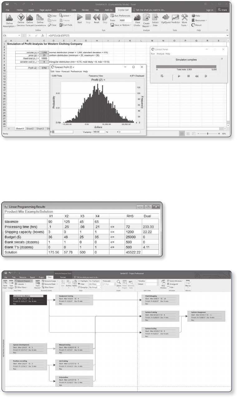
Crystal Ball
Another spreadsheet add-
in program is Crystal Ball
by Oracle. Crystal Ball is
demonstrated in Chap
-
ter 14 on simulation and
shows how to perform
simulation analysis for
certain types of risk anal
-
ysis and forecasting prob-
lems. Here is an example
of one of the Crystal Ball
files (from Chapter 14)
that is on the Companion
Web site. The Compan
-
ion Web site will direct
you to a trial version of
the software.
QM for Windows Software Package
QM for Windows is a computer package that is included on the text Companion Web site, and
many students and instructors will prefer to use it with this text. This software is very user-
friendly, requiring virtually no preliminary instruction except for the “help” screens that can be
accessed directly from the program. It is demonstrated throughout the text in conjunction with
virtually every management science modeling technique, except simulation. The text includes
50 QM for Windows screens used to demonstrate
example problems. Thus, for most topics problem
solution is demonstrated via both Excel spreadsheets
and QM for Windows. Files that include all the QM
for Windows solutions, for example, in the text are
included on the accompanying Companion Web site.
Here is an example of one of the QM for Windows
files (from Chapter 4 on linear programming) that is
on the Companion Web site.
Microsoft Project
Chapter 8 on project
management includes the
popular software package
Microsoft Project. Here is
an example of one of the
Microsoft Project files
(from Chapter 8) that
is available on the text
Companion Web site. The
Companion Web site will
direct you to a trial ver-
sion of the software.
16 PREFACE
A01_TAYL3045_13_GE_FM.indd 16 29/10/2018 16:50

Problems and Cases
Previous editions of the text always provided a substantial number of homework questions,
problems, and cases for students to practice on. This edition includes more than 800 homework
problems, 20 of which are new, and 69 end-of-chapter case problems.
Marginal Notes
Notes in the margins of this text serve the same basic
function as notes that students themselves might write
in the margin. They highlight certain topics to make it
easier for students to locate them, summarize topics and
important points, and provide brief definitions of key
terms and concepts.
Examples
The primary means of teaching the various quanti-
tative modeling techniques presented in this text is
through examples. Thus, examples are liberally inserted
throughout the text, primarily to demonstrate how prob-
lems are solved with the different quantitative tech-
niques and to make them easier to understand. These
examples are organized in a logical step-by-step solu-
tion approach that the student can subsequently apply
to the homework problems.
Example Problem Solutions
At the end of each chapter, just prior to the home-
work questions and problems, is a section that pro-
vides solved examples to serve as a guide for doing the
homework problems. These examples are solved in a
detailed, step-by-step fashion. Here is an example from
Chapter 2.
Chapter Web Links
The files on the Companion Web site contains Chapter
Web links for every chapter in the text. These Web links
access tutorials, summaries, and notes available on the
Internet for the various techniques and topics in every
chapter in the text. Also included are YouTube videos
that provide additional learning resources and tutorials
about many of the topics and techniques, links to the
development and developers of the techniques in the
text, and links to the Web sites for the companies and
organizations that are featured in the “Management Sci-
ence Application” boxes in every chapter. The “Chapter
Web links” file includes more than 550 Web links.
PREFACE 17
A01_TAYL3045_13_GE_FM.indd 17 29/10/2018 16:50
Chapter Modules
Several of the strictly mathematical topics—such as the simplex and transportation solution
methods—are included as chapter modules on the Companion Web site, at http://www.pearson
globaleditions.com
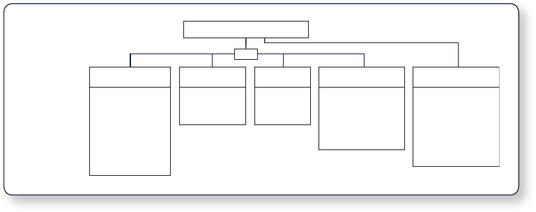
Table of Contents Overview
An important objective is to have a well-organized text that flows smoothly and follows a logi-
cal progression of topics, placing the different management science modeling techniques in their
proper perspective. The following Figure 1.6 from Chapter 1 outlines the organization of topics
in the book.
The first 10 chapters are related to mathematical programming that can be solved using
Excel spreadsheets, including linear, integer, nonlinear, and goal programming, as well as network
techniques.
Within these math-
ematical programming
chapters, the traditional
simplex procedure for
solving linear program-
ming problems math-
ematically is located
in Module A on the
Companion Web site,
at http://www.pearson
globaleditions.com, that
accompanies this text. It
can still be covered by
the student on the com-
puter as part of linear
programming, or it can be
excluded, without leaving
a “hole” in the presentation of this topic. The integer programming mathematical branch and
bound solution method (Chapter 5) is located in Module C on the Companion Web site. In Chapter
6, on the transportation and assignment problems, the strictly mathematical solution approaches,
including the northwest corner, VAM, and stepping-stone methods, are located in Module B on
the Companion Web site. Because transportation and assignment problems are specific types of
network problems, the two chapters that cover network flow models and project networks that can
be solved with linear programming, as well as traditional model-specific solution techniques and
software, follow Chapter 6 on transportation and assignment problems. In addition, in Chapter
10, on nonlinear programming, the traditional mathematical solution techniques, including the
substitution method and the method of Lagrange multipliers, are located in Module D on the
Companion Web site.
Chapters 11 through 14 include topics generally thought of as being probabilistic, includ-
ing probability and statistics, decision analysis, queuing, and simulation. Module F on Markov
analysis and Module E on game theory are on the Companion Web site. Forecasting in
Chapter15 and inventory management in Chapter 16 are both unique topics related to opera-
tions management.
16 Chapter 1 ManageMent SCienCe
a list of all the model solution modules available in QM for Windows. Clicking on the “Break-
even Analysis” module will access a new screen for typing in the problem title. Clicking again
will access a screen with input cells for the model parameters—that is, fixed cost, variable cost,
and price (or revenue). Next, clicking on the “Solve” button at the top of the screen will provide
the solution and the break-even graph for the Western Clothing Company example, as shown in
Exhibit 1.3.
Management Science Modeling Techniques
This text focuses primarily on two of the five steps of the management science process described
in Figure 1.1—model construction and solution. These are the two steps that use the manage-
ment science techniques. In a textbook, it is difficult to show how an unstructured real-world
problem is identified and defined because the problem must be written out. However, once a
problem statement has been given, we can show how a model is constructed and a solution is
derived. The techniques presented in this text can be loosely classified into four categories, as
shown in Figure 1.6.
EXHIBIT 1.3
FIGURE 1.6
Classification
of management
science
techniques
Management science techniques
Probabilistic
techniques
Linear mathematical
programming
Linear programming
models
Graphical analysis
Sensitivity analysis
Transportation,
transshipment,
and assignment
Integer linear
programming
Goal programming
Decision analysis
Probability and
statistics
Queuing
Network
Text
techniques
Network flow
Project
management
(CPM/PERT)
Other techniques
Forecasting
Simulation
Inventory
Analytical hierarchy
process (AHP)
Nonlinear
programming
Companion Web site
Branch and bound
Markov analysis
Game theory
method
Simplex method
Transportation
and assignment
methods
Nonlinear programming
Linear Mathematical Programming Techniques
Chapters 2 through 6 and 9 present techniques that together make up linear mathematical program-
ming. (The first example used to demonstrate model construction earlier in this chapter is a very
rudimentary linear programming model.) The term programming used to identify this technique
M01_TAYL0660_13_SE_C01.indd 16 8/21/17 2:36 PM
18 PREFACE
A01_TAYL3045_13_GE_FM.indd 18 29/10/2018 16:50

Instructor Teaching Resources
This text comes with the following teaching resources.
Supplements available to instructors at
http://www.pearsonglobaleditions.com
Features of the Supplement
Instructor's Solutions Manual developed by
the author
•
Detailed solutions for all end-of-chapter
exercises and cases
•
One file per chapter provided in MS Word
format
Excel Homework Solutions developed by the
author
•
A corresponding Excel solution file for
almost all 840 end-of-chapter homework and
case problems in the text
•
Organized by chapter and problem number
•
Also includes Excel homework solution files
for TreePlan, Crystal Ball, and Microsoft
Project
Test Bank authored by Geoff Willis of the
University of Central Oklahoma
•
2,000 questions, including true/false,
multiple-choice, and problem-solving
questions for each chapter
•
Each question followed by the correct answer,
page references, main headings, difficulty
rating, and key words
TestGen
®
Computerized Test Bank
•
Pearson Education's test-generating
software, PC and Mac compatible, and
preloaded with all of the Test Bank questions
•
Can manually or randomly view test
questions and drag and drop to create a test
•
Can add or modify test bank questions as
needed
PowerPoint Presentations authored by Geoff
Willis of the University of Central Oklahoma
•
Available for every chapter
•
Features figures, tables, Excel spreadsheets,
and main points
•
They meet accessibility standards for
students with disabilities. Features include,
but not limited to:
∘
Keyboard and Screen Reader access
∘
Alternative text for images
∘
High color contrast between background
and foreground colors
Chapter Web Links developed by the author
•
Internet links to tutorials, summaries, notes
and videos
Acknowledgments
As with any other large project, the revision of a textbook is not accomplished without the help of
many people. The 13th edition of this book is no exception, and I would like to take this oppor-
tunity to thank those who have contributed to its preparation.
I thank the reviewers of this and previous editions: Dr. B. S. Bal, Nagraj Balakrishnan,
Edward M. Barrow, Ali Behnezhad, Weldon J. Bowling, Rod Carlson, Petros Christofi, Yar
M.Ebadi, Richard Ehrhardt, Warren W. Fisher, James Flynn, Wade Furgeson, Soumen Ghosh,
PREFACE 19
A01_TAYL3045_13_GE_FM.indd 19 29/10/2018 16:50
James C. Goodwin, Jr., Richard Gunther, Dewey Hemphill, Ann Hughes, Shivaji Khade, David
A. Larson, Sr., Shao-ju Lee, Robert L. Ludke, Peter A. Lyew, Robert D. Lynch, Dinesh Manocha,
Mildred Massey, Russell McGee, Abdel-Aziz Mohamed, Anthony Narsing, Thomas J. Nolan,
Susan W. Palocsay, David W. Pentico, Cindy Randall, Christopher M. Rump, Michael E. Salassi,
Roger Schoenfeldt, Jaya Singhal, Charles H. Smith, Lisa Sokol, Daniel Solow, Dothang Truong,
John Wang, Edward Williams, Barry Wray, Kefeng Xu, Hulya Julie Yazici, Ding Zhang, and
Zuopeng Zhang.
I am also very grateful to Tracy McCoy at Virginia Tech for her valued assistance. I would
like to thank my Content Producer, Sugandh Juneja, at Pearson, for her valuable assistance and
patience. I very much appreciate the help and hard work of Roberta Sherman and all the folks at
SPi Global, who produced this edition, and the text’s accuracy checker, M. Khurrum S. Bhutta.
Finally, I would like to thank my editors, Dan Tylman and Neeraj Bhalla, at Pearson, for their
continued help and patience.
Global Edition Acknowledgments
Pearson would like to thank the following people for their contribution to the Global Edition:
Contributors:
Ahmed ElMelegy, Gulf University for Science and Technology
Subramaniam Ponnaiyan, American University in Dubai
Reviewers:
Ahmed ElMelegy, Gulf University for Science and Technology
Ipek Seriyan Topan, University of Twente
20 PREFACE
A01_TAYL3045_13_GE_FM.indd 20 29/10/2018 16:50

21
Chapter
Management Science
1
M01_TAYL3045_13_GE_C01.indd 21 26/10/2018 09:41
22 Chapter 1 ManageMent SCienCe
Management science is the application of a scientific approach to solving management prob-
lems to help managers make better decisions. As implied by this definition, management science
encompasses a number of mathematically oriented techniques that have either been developed
within the field of management science or been adapted from other disciplines, such as the natu-
ral sciences, mathematics, statistics, and engineering. This text provides an introduction to the
techniques that make up management science and demonstrates their applications to management
problems.
Management science is a recognized and established discipline in business. The applications
of management science techniques are widespread, and they have been frequently credited with
increasing the efficiency and productivity of business firms. In various surveys of businesses,
many indicate that they use management science techniques, and most rate the results to be very
good. Management science (also referred to as operations research, quantitative methods, quan-
titative analysis, decision sciences, and business analytics) is part of the fundamental curriculum
of most programs in business.
As you proceed through the various management science models and techniques contained
in this text, you should remember several things. First, most of the examples presented in this text
are for business organizations because businesses represent the main users of management sci-
ence. However, management science techniques can be applied to solve problems in different
types of organizations, including services, government, military, business and industry, and health
care.
Second, in this text all the modeling techniques and solution methods are mathematically
based. In some instances the manual, mathematical solution approach is shown because it helps
one understand how the modeling techniques are applied to different problems. However, a com-
puter solution is possible for each of the modeling techniques in this text, and in many cases the
computer solution is emphasized. The more detailed mathematical solution procedures for many
of the modeling techniques are included as supplemental modules on the companion Web site
for this text.
Finally, as the various management science techniques are presented, keep in mind that
management science is more than just a collection of techniques. Management science also
involves the philosophy of approaching a problem in a logical manner (i.e., a scientific
approach). The logical, consistent, and systematic approach to problem solving can be as
useful (and valuable) as the knowledge of the mechanics of the mathematical techniques
themselves. This understanding is especially important for those readers who do not always
see the immediate benefit of studying mathematically oriented disciplines such as manage-
ment science.
The Management Science Approach to Problem Solving
As indicated in the previous section, management science encompasses a logical, systematic
approach to problem solving, which closely parallels what is known as the scientific method for
attacking problems. This approach, as shown in Figure 1.1, follows a generally recognized and
ordered series of steps: (1) observation, (2) definition of the problem, (3) model construction,
(4)model solution, and (5) implementation of solution results. We will analyze each of these steps
individually in this text.
Observation
The first step in the management science process is the identification of a problem that exists in
the system (organization). The system must be continuously and closely observed so that prob-
lems can be identified as soon as they occur or are anticipated. Problems are not always the result
of a crisis that must be reacted to but, instead, frequently involve an anticipatory or planning
situation. The person who normally identifies a problem is the manager because managers work
in places where problems might occur. However, problems can often be identified by a
Management
science is a scientific
approach to solving
management
problems.
Management
science can be
used in a variety of
organizations to solve
many different types
of problems.
Management science
encompasses a logical
approach to problem
solving.
The steps of the
scientific method
are(1) observation,
(2) problem definition,
(3) model construction,
(4) model solution, and
(5) implementation.
M01_TAYL3045_13_GE_C01.indd 22 26/10/2018 09:41

the ManageMent SCienCe approaCh to probleM Solving 23
management scientist, a person skilled in the techniques of management science and trained to
identify problems, who has been hired specifically to solve problems using management science
techniques.
Definition of the Problem
Once it has been determined that a problem exists, the problem must be clearly and concisely
defined. Improperly defining a problem can easily result in no solution or an inappropriate solu-
tion. Therefore, the limits of the problem and the degree to which it pervades other units of the
organization must be included in the problem definition. Because the existence of a problem
implies that the objectives of the firm are not being met in some way, the goals (or objectives) of
the organization must also be clearly defined. A stated objective helps to focus attention on what
the problem actually is.
Model Construction
A management science model is an abstract representation of an existing problem situation. It
can be in the form of a graph or chart, but most frequently a management science model consists
of a set of mathematical relationships. These mathematical relationships are made up of numbers
and symbols.
As an example, consider a business firm that sells a product. The product costs $5 to
produce and sells for $20. A model that computes the total profit that will accrue from the
items sold is
Z = +20x - 5x
In this equation, x represents the number of units of the product that are sold, and Z represents the
total profit that results from the sale of the product. The symbols x and Z are variables. The term
variable is used because no set numeric value has been specified for these items. The number of
units sold, x, and the profit, Z, can be any amount (within limits); they can vary. These two vari-
ables can be further distinguished. Z is a dependent variable because its value is dependent on the
number of units sold; x is an independent variable because the number of units sold is not depen-
dent on anything else (in this equation).
The numbers $20 and $5 in the equation are referred to as parameters. Parameters are
constant values that are generally coefficients of the variables (symbols) in an equation.
A management
scientist is a
person skilled in
the application of
management science
techniques.
A model is an
abstract mathematical
representation of a
problem situation.
A variable is a symbol
used to represent an
item that can take on
any value.
Parameters are known,
constant values that
are often coecients of
variables in equations.
FIGURE 1.1
The management
science process
Management
science
techniques
Observation
Problem
definition
Model
construction
Solution
Feedback
Information
Implementation
M01_TAYL3045_13_GE_C01.indd 23 26/10/2018 09:41
24 Chapter 1 ManageMent SCienCe
Parameters usually remain constant during the process of solving a specific problem. The param-
eter values are derived from data (i.e., pieces of information) from the problem environment.
Sometimes the data are readily available and quite accurate. For example, presumably the selling
price of $20 and product cost of $5 could be obtained from the firm’s accounting department and
would be very accurate. However, sometimes data are not as readily available to the manager or
firm, and the parameters must be either estimated or based on a combination of the available data
and estimates. In such cases, the model is only as accurate as the data used in constructing the
model.
The equation as a whole is known as a functional relationship (also called function and
relationship). The term is derived from the fact that profit, Z, is a function of the number of units
sold, x, and the equation relates profit to units sold.
Because only one functional relationship exists in this example, it is also the model. In this
case, the relationship is a model of the determination of profit for the firm. However, this model
does not really replicate a problem. Therefore, we will expand our example to create a problem
situation.
Let us assume that the product is made from steel and that the business firm has 100 pounds
of steel available. If it takes 4 pounds of steel to make each unit of the product, we can develop
an additional mathematical relationship to represent steel usage:
4x = 100 lb. of steel
This equation indicates that for every unit produced, 4 of the available 100 pounds of steel
will be used. Now our model consists of two relationships:
Z = +20x - 5x
4x = 100
We say that the profit equation in this new model is an objective function, and the resource
equation is a constraint. In other words, the objective of the firm is to achieve as much profit, Z,
as possible, but the firm is constrained from achieving an infinite profit by the limited amount
of steel available. To signify this distinction between the two relationships in this model, we will
add the following notations:
maximize Z = +20x - 5x
subject to
4x = 100
This model now represents the manager’s problem of determining the number of units to
produce. You will recall that we defined the number of units to be produced as x. Thus, when we
determine the value of x, it represents a potential (or recommended) decision for the manager.
Therefore, x is also known as a decision variable. The next step in the management science pro-
cess is to solve the model to determine the value of the decision variable.
Model Solution
Once models have been constructed in management science, they are solved using the man-
agement science techniques presented in this text. A management science solution technique
usually applies to a specific type of model. Thus, the model type and solution method are
both part of the management science technique. We are able to say that a model is solved
because the model represents a problem. When we refer to model solution, we also mean
problem solution.
Data are pieces of
information from the
problem environment.
A model is a
functional
relationship that
includes variables,
parameters, and
equations.
A management
science technique
usually applies to a
specific model type.
M01_TAYL3045_13_GE_C01.indd 24 26/10/2018 09:41

the ManageMent SCienCe approaCh to probleM Solving 25
For the example model developed in the previous section,
maximize Z = +20x - 5x
subject to
4x = 100
the solution technique is simple algebra. Solving the constraint equation for x, we have
4x = 100
x = 100/4
x = 25 units
Substituting the value of 25 for x into the profit function results in the total profit:
Z = +20x - 5x
= 20(25) - 5(25)
= +375
Thus, if the manager decides to produce 25 units of the product and all 25 units sell, the busi-
ness firm will receive $375 in profit. Note, however, that the value of the decision variable does
not constitute an actual decision; rather, it is information that serves as a recommendation or
guideline, helping the manager make a decision.
Some management science techniques do not generate an answer or a recommended deci-
sion. Instead, they provide descriptive results: results that describe the system being modeled. For
A management
sciencesolution
can be either a
recommended decision
or information that
helps a manager
makea decision.
Time Out for Pioneers in Management Science
t
hroughout this text, TIME OUT boxes introduce you to
the individuals who developed the various techniques that
are described in the chapters. This provides a historical
perspective on the development of the field of management
science. In this first instance, we will briefly outline the develop-
ment of management science.
Although a number of the mathematical techniques that
make up management science date to the turn of the twentieth
century or before, the field of management science itself can
trace its beginnings to military operations research (OR) groups
formed during World War II in Great Britain circa 1939. These OR
groups typically consisted of a team of about a dozen individuals
from different fields of science, mathematics, and the military,
brought together to find solutions to military-related problems.
One of the most famous of these groups—called “Blackett’s
circus” after its leader, Nobel Laureate P. M. S. Blackett of the
University of Manchester and a former naval officer—included
three physiologists, two mathematical physicists, one astrophysi-
cist, one general physicist, two mathematicians, an Army officer,
and a surveyor. Blackett’s group and the other OR teams made
significant contributions in improving Britain’s early-warning
radar system (which was instrumental in their victory in the
Battle of Britain), aircraft gunnery, antisubmarine warfare, civil-
ian defense, convoy size determination, and bombing raids over
Germany.
The successes achieved by the British OR groups were
observed by two Americans working for the U.S. military,
Dr.James B. Conant and Dr. Vannevar Bush, who recommended
that OR teams be established in the U.S. branches of the military.
Subsequently, both the Air Force and Navy created OR groups.
After World War II, the contributions of the OR groups were
considered so valuable that the Army, Air Force, and Navy set
up various agencies to continue research of military problems.
Two of the more famous agencies were the Navy’s Operations
Evaluation Group at MIT and Project RAND, established by the
Air Force to study aerial warfare. Many of the individuals who
developed OR and management science techniques did so while
working at one of these agencies after World War II or as a result
of their work there.
As the war ended and the mathematical models and
techniques that were kept secret during the war began to be
released, there was a natural inclination to test their applicabil-
ity to business problems. At the same time, various consulting
firms were established to apply these techniques to industrial
and business problems, and courses in the use of quantitative
techniques for business management began to surface in Ameri-
can universities. In the early 1950s, the use of these quantitative
techniques to solve management problems became known as
management science, and it was popularized by a book of that
name by Stafford Beer of Great Britain.
M01_TAYL3045_13_GE_C01.indd 25 26/10/2018 09:41

26 Chapter 1 ManageMent SCienCe
example, suppose the business firm in our example desires to know the average number of units
sold each month during a year. The monthly data (i.e., sales) for the past year are as follows:
Month Sales Month Sales
January 30 July 35
February 40 August 50
March 25 September 60
April 60 October 40
May 30 November 35
June 25 December
50
Total 480 units
Monthly sales average 40 units
(480 , 12).
This result is not a decision; it is information
that describes what is happening in the system. The results of the management science techniques
Management Science Application
Room Pricing with Management Science and Analytics at Marriott
inventory is given to a group rather than being held for indi-
vidual bookings.
To address the group booking process, Marriott developed
a decision support system, Group Pricing Optimizer (GPO), that
provides guidance to Marriott personnel on pricing hotel rooms
for group customers. GPO uses various management science
modeling techniques and tools, including simulation, forecast-
ing, and optimization techniques, to recommend an optimal
price rate. Marriott estimates that GPO provided an improve-
ment in profit of over $120 million derived from $1.3 billion in
group business in its first 2 years of use.
Source: Based on S. Hormby, J. Morrison, P. Dave, M. Myers, and T.
Tenca, “Marriott International Increases Revenue by Implementing a Group
Pricing Optimizer,” Interfaces 40, no. 1 (January–February 2010): 47–57.
M
arriott International, Inc., headquartered in Bethesda,
Maryland, has more than 140,000 employees work-
ing at more than 3,300 hotels in 70 countries. Its
hotel franchises include Marriott, JW Marriott, The Ritz-Carlton,
Renaissance, Residence Inn, Courtyard, TownePlace Suites, Fair-
field Inn, and Springhill Suites. Fortune magazine ranks Marriott
as the lodging industry’s most admired company and one of the
best companies to work for.
Marriott uses a revenue management system for individual
hotel bookings. This system provides forecasts of customer
demand and pricing controls, makes optimal inventory alloca-
tions, and interfaces with a reservation system that handles
more than 75 million transactions each year. The system
makes a demand forecast for each rate category and length
of stay for each arrival day up to 90 days in advance, and it
provides inventory allocations to the reservation system. This
inventory of hotel rooms is then sold to individual custom-
ers through channels such as Marriott.com, the company’s
toll-free reservation number, the hotels directly, and global
distribution systems.
One of the most significant revenue streams for Marriott
is for group sales, which can contribute more than half of
a full-service hotel’s revenue. However, group business has
challenging characteristics that introduce uncertainty and
make modeling it difficult, including longer booking win-
dows (as compared to those for individuals), price negotia-
tion as part of the booking process, demand for blocks of
rooms, and lack of demand data. For a group request, a
hotel must know if it has sufficient rooms and determine
a recommended rate. A key challenge is estimating the
value of the business the hotel is turning away if the room
David Zanzinger/Alamy Stock Photo
M01_TAYL3045_13_GE_C01.indd 26 26/10/2018 09:41
ManageMent SCienCe and buSineSS analytiCS 27
in this text are examples of the two types shown in this section: (1) solutions/ decisions and
(2)descriptive results.
Implementation
The final step in the management science process for problem solving described in Figure 1.1 is
implementation. Implementation is the actual use of the model once it has been developed or the
solution to the problem the model was developed to solve. This is a critical but often overlooked
step in the process. It is not always a given that once a model is developed or a solution found, it
is automatically used. Frequently the person responsible for putting the model or solution to use
is not the same person who developed the model, and thus the user may not fully understand how
the model works or exactly what it is supposed to do. Individuals are also sometimes hesitant to
change the normal way they do things or to try new things. In this situation, the model and solu-
tion may get pushed to the side or ignored altogether if they are not carefully explained and their
benefit fully demonstrated. If the management science model and solution are not implemented,
then the effort and resources used in their development have been wasted.
Management Science and Business Analytics
Analytics is the latest hot topic and new buzzword in business. Companies are establishing ana-
lytics departments, and the demand for employees with analytics skills and expertise is growing
faster than almost any other business skill set. Universities and business schools are developing
new degree programs and courses in analytics. So exactly what is this new and very popular area
called business analytics, and how does it relate to management science?
Business analytics is a somewhat general term that seems to have a number of different defi-
nitions, but in broad terms it is considered to be a process for using large amounts of data com-
bined with information technology, statistics, management science techniques, and mathematical
modeling to help managers solve problems and make decisions that will improve their business
performance. It makes use of these technological tools to help businesses understand their past
performance and to help them plan and make decisions for the future; thus analytics is said to be
descriptive, predictive, and prescriptive.
Much as the word science groups together a number of disciplines such as chemistry, biol-
ogy, physics, geology, and so on, the word analytics seems to group together disciplines such as
management science, operations research, statistics, computer science, engineering, data science,
and so on. All of these disciplines (and thus analytics, in general) have in common the scientific
method for addressing problems that was discussed in the previous section.
A key component of business analytics is the recent availability of large amounts of data—called
“big data”—that is now accessible to businesses, and that is perceived to be an integral part and starting
point of the analytical process. Data are considered to be the engine that drives the process of analysis
and decision making in business analytics. For example, a bank might apply analytics by using data
to determine different customer characteristics to match them with the bank services they provide; or
a retail store might apply analytics by using data to determine which styles of denim jeans match their
customer preferences, determine how many jeans to order from their foreign suppliers, how much
inventory to keep on hand, and when the best time is to sell the jeans and what is the best price.
If you have not already noticed, analytics is very much like the “management science approach
to problem solving” that we have already described in the previous section. In fact, many in busi-
ness perceive business analytics to just be a repackaged version of management science. In some
business schools, management science courses are simply being renamed as “analytics.” Business
students are being advised that in the future companies will expect them to have an analytics skill
set, and these skills need to include knowledge of statistics, mathematical modeling, and quantitative
tools—the topics traditionally considered to be management science and that are covered in this text.
For our purposes in studying management science, it is clear that the quantitative tools and
techniques that are included in this book are an important major part of business analytics, no
Implementation is the
actual use of a model
once it has been
developed.
Business analytics
uses large amounts
of data with
management science
techniques and
modeling to help
managers makes
decisions.
M01_TAYL3045_13_GE_C01.indd 27 26/10/2018 09:41
28 Chapter 1 ManageMent SCienCe
matter what the definition of the business analytics process is. As such, becoming skilled in the
use of these management science techniques is a necessary and important step for someone who
wants to become a business analytics professional.
Developing Analytical Career Skills
As you learn the management science techniques in this text, you may think that they are not rel-
evant to what you imagine your future job might be. However, you can be assured that this is not
the case. Whether or not you plan on a career in which management science or business analytics
is a key part, the logical, analytical approach to problem solving and decision making employed
in management science will help you in any career path you choose. It is through the aggregate
of your educational experiences that you will develop the skills that employers have identified as
critical to success in the workplace.
Management science provides students with many of these skill sets besides just the
quantitative techniques it comprises that employers will seek and value in business graduates
who market themselves as having expertise in business analytics. The ability to bring critical
thinking to problem-solving scenarios is an important aspect of business analytics, which
management science provides. Critical thinking involves purposeful and goal directed think-
ing used to define and solve problems, make decisions and form judgements related to a
particular situation or set of circumstances. This is what management science does by provid-
ing a structured format for looking at problems and defining them, formulating them as
mathematical models, and providing approaches to solving them that result in decisions that
achieve the organization’s goals.
Many decision-making scenarios take place in a project team-based environment where
collaboration is a necessary skill. Management science provides an approach to problem
solving in which individuals may actively work together on a problem using their combined
efforts to construct meaning and knowledge as a group through dialogue and negotiation that
ultimately results in a modeling approach that reflects their joint actions. Chapter 8 on “Proj-
ect Management” directly addresses this collaborative project-based approach to decision
making.
Because of its reliance on computer software to solve decision problems that students
will learn about in this text, management science teaches information technology and com-
puting skills that are very important to employers. Implicit in the management science
approach is the ability to select and use the appropriate technology to solve a particular type
of modeling problem. The student of management science learns how to apply computing
skills to solve problems and show proficiency with the various computer software programs
introduced in the text, including Excel, QM for Windows, MS Project, Crystal Ball, and
Treeplan, among others.
We have already noted the importance of data in business analytics, and management science
provides a platform for a student to develop data literacy, the ability to access, interpret, manipu-
late, summarize, and communicate data in a decision-making situation.
Model Building: Break-Even Analysis
In the previous section, we gave a brief, general description of how management science models
are formulated and solved, using a simple algebraic example. In this section, we will continue
toexplore the process of building and solving management science models, using break-even
analysis, alsocalled profit analysis. Break-even analysis is a good topic to expand our discussion
of model building and solution because it is straightforward, relatively familiar to most people,
and not overly complex. In addition, it provides a convenient means to demonstrate the different
ways management science models can be solved—mathematically (by hand), graphically, and
with a computer.
Critical thnking
purpsoeful and goal
directed thinking
used to define and
solve problems, make
decsions and form
judgements related to
a particular situation.
Collaboration a
necessary skill for
decision scenarios
that take place in a
project team-based
environment.
Information
technology and
computing skills
important attributes
to employers because
of the reliance on
computer software
to solve decison
problems.
Data Literacy the
ability to acccess,
interpret, manipulate,
summarize and
commnicte data in
a decison-making
situation.
Break-even analysis is
a modeling technique
to determine the
number of units to sell
or produce that will
result in zero profit.
M01_TAYL3045_13_GE_C01.indd 28 26/10/2018 09:41
Model building: break-even analySiS 29
The purpose of break-even analysis is to determine the number of units of a product (i.e.,
the volume) to sell or produce that will equate total revenue with total cost. The point where total
revenue equals total cost is called the break-even point, and at this point profit is zero. The break-
even point gives a manager a point of reference in determining how many units will be needed
to ensure a profit.
Components of Break-Even Analysis
The three components of break-even analysis are volume, cost, and profit. Volume is the level
of sales or production by a company. It can be expressed as the number of units (i.e., quantity)
produced and sold, as the dollar volume of sales, or as a percentage of total capacity available.
Two types of cost are typically incurred in the production of a product: fixed costs and vari-
able costs. Fixed costs are generally independent of the volume of units produced and sold. That
is, fixed costs remain constant, regardless of how many units of product are produced within a
given range. Fixed costs can include such items as rent on plant and equipment, taxes, staff and
management salaries, insurance, advertising, depreciation, heat and light, and plant maintenance.
Taken together, these items result in total fixed costs.
Variable costs are determined on a per-unit basis. Thus, total variable costs depend on the
number of units produced. Variable costs include such items as raw materials and resources, direct
labor, packaging, material handling, and freight.
Total variable costs are a function of the volume and the variable cost per unit. This relation-
ship can be expressed mathematically as
total variable cost = vc
v
where
c
v
= variable cost per unit
and
v = volume
(number of units) sold.
The total cost of an operation is computed by summing total fixed cost and total variable
cost, as follows:
total cost = total fixed cost + total variable cost
or
TC = c
f
+ vc
v
where
c
f
= fixed cost.
As an example, consider Western Clothing Company, which produces denim jeans. The
company incurs the following monthly costs to produce denim jeans:
fixed cost = c
f
= +10,000
variable cost = c
v
= +8 per pair
If we arbitrarily let the monthly sales volume, v, equal 400 pairs of denim jeans, the total cost is
TC = c
f
+ vc
v
= +10,000 + (400)(8) = +13,200
The third component in our break-even model is profit. Profit is the difference between total
revenue and total cost. Total revenue is the volume multiplied by the price per unit,
total revenue = vp
where
p = price per unit.
Fixed costs are
independent of
volume and remain
constant.
Variable costs depend
on the number of
items produced.
Total cost (TC) equals
the fixed cost
(c
f
)
plus
the variable cost per
unit
(c
v
)
multiplied by
volume (v).
Profit is the difference
between total revenue
(volume multiplied by
price) and total cost.
M01_TAYL3045_13_GE_C01.indd 29 26/10/2018 09:41
30 Chapter 1 ManageMent SCienCe
For our clothing company example, if denim jeans sell for $23 per pair and we sell 400 pairs
per month, then the total monthly revenue is
total revenue = vp = (400)(23) = +9,200
Now that we have developed relationships for total revenue and total cost, profit (Z) can be
computed as follows:
total profit = total revenue - total cost
Z = vp - (c
f
+ vc
v
)
= vp - c
f
- vc
v
Computing the Break-Even Point
For our clothing company example, we have determined total revenue and total cost to be
$9,200 and $13,200, respectively. With these values, there is no profit but, instead, a loss of
$4,000:
total profit = total revenue - total cost = +9,200 - 13,200 = -+4,000
We can verify this result by using our total profit formula,
Z = vp - c
f
- vc
v
and the values
v = 400,
p = +23,
c
f
= +10,000,
and
c
v
= +8:
Z = vp - c
f
- vc
v
= +(400)(23) - 10,000 - (400)(8)
= +9,200 - 10,000 - 3,200
= -+4,000
Obviously, the clothing company does not want to operate with a monthly loss of $4,000
because doing so might eventually result in bankruptcy. If we assume that price is static because of
market conditions and that fixed costs and the variable cost per unit are not subject to change, then
the only part of our model that can be varied is volume. Using the modeling terms we developed
earlier in this chapter, price, fixed costs, and variable costs are parameters, whereas the volume,
v, is a decision variable. In break-even analysis, we want to compute the value of v that will result
in zero profit.
At the break-even point, where total revenue equals total cost, the profit, Z, equals zero.
Thus, if we let profit, Z, equal zero in our total profit equation and solve for v, we can determine
the break-even volume:
Z = vp - c
f
- vc
v
0 = v(23) - 10,000 - v(8)
0 = 23v - 10,000 - 8v
15v = 10,000
v = 666.7 pairs of jeans
In other words, if the company produces and sells 666.7 pairs of jeans, the profit (and loss)
will be zero, and the company will break even. This gives the company a point of reference
from which to determine how many pairs of jeans it needs to produce and sell to gain a profit
The break-even point
is the volume (v) that
equates total revenue
with total cost where
profit is zero.
M01_TAYL3045_13_GE_C01.indd 30 26/10/2018 09:41

Model building: break-even analySiS 31
(subject to any capacity limitations). For example, a sales volume of 800 pairs of denim jeans
will result in the following monthly profit:
Z = vp - c
f
- vc
v
= +(800)(23) - 10,000 - (800)(8) = +2,000
In general, the break-even volume can be determined using the following formula:
Z = vp - c
f
- vc
v
0 = v(p - c
v
) - c
f
v(p - c
v
) = c
f
v =
c
f
p - c
v
For our example,
v
=
c
f
p - c
v
=
10,000
23 - 8
= 666.7 pairs of jeans
Graphical Solution
It is possible to represent many of the management science models in this text graphically and use
these graphical models to solve problems. Graphical models also have the advantage of provid-
ing a “picture” of the model that can sometimes help us understand the modeling process better
than mathematics alone can. We can easily graph the break-even model for our Western Clothing
Company example because the functions for total cost and total revenue are linear. That means
we can graph each relationship as a straight line on a set of coordinates, as shown in Figure 1.2.
FIGURE 1.2
Break-even model
10
20
30
40
50
200
0
400 600 800 1,000 1,200
1,400 1,600
Volume, v
Total cost
Revenue, cost,
and profit ($1,000s)
Variable cost
Fixed cost
Total revenue
Loss
Profit
Break-even
point
In Figure 1.2, the fixed cost,
c
f
,
has a constant value of $10,000, regardless of the volume. The
total cost line, TC, represents the sum of variable cost and fixed cost. The total cost line increases
because variable cost increases as the volume increases. The total revenue line also increases as
volume increases, but at a faster rate than total cost. The point where these two lines intersect
indicates that total revenue equals total cost. The volume, v, that corresponds to this point is the
break-even volume. The break-even volume in Figure 1.2 is 666.7 pairs of denim jeans.
Sensitivity Analysis
We have now developed a general relationship for determining the break-even volume, which
was the objective of our modeling process. This relationship enables us to see how the level of
profit (and loss) is directly affected by changes in volume. However, when we developed this
M01_TAYL3045_13_GE_C01.indd 31 26/10/2018 09:41

32 Chapter 1 ManageMent SCienCe
model, we assumed that our parameters, fixed and variable costs and price, were constant. In
reality such parameters are frequently uncertain and can rarely be assumed to be constant, and
changes in any of the parameters can affect the model solution. The study of changes on a man-
agement science model is called sensitivity analysis—that is, seeing how sensitive the model is
to changes.
Sensitivity analysis can be performed on all management science models in one form or
another. In fact, sometimes companies develop models for the primary purpose of experimenta-
tion to see how the model will react to different changes the company is contemplating or that
management might expect to occur in the future. As a demonstration of how sensitivity analysis
works, we will look at the effects of some changes on our break-even model.
The first thing we will analyze is price. As an example, we will increase the price for denim
jeans from $23 to $30. As expected, this increases the total revenue, and it therefore reduces the
break-even point from 666.7 pairs of jeans to 454.5 pairs of jeans:
v
=
c
f
p - c
v
=
10,000
30 - 8
= 454.5 pairs of denim jean
s
The effect of the price change on break-even volume is illustrated in Figure 1.3.
Sensitivity analysis
sees how sensitive a
management model is
to changes.
In general, an
increase in price
lowers the break-even
point, all other things
held constant.
FIGURE 1.3
Break-even model
with an increase
in price
10
20
30
40
50
200
0
400 600 800 1,000 1,200
1,400 1,600
Volume, v
Total cost
Revenue, cost,
and profit ($1,000s)
New total
revenue
Fixed cost
Old total
revenue
Old B-E point
New B-E point
Although a decision to increase price looks inviting from a strictly analytical point of view,
it must be remembered that the lower break-even volume and higher profit are possible but not
guaranteed. A higher price can make it more difficult to sell the product. Thus, a change in price
often must be accompanied by corresponding increases in costs, such as those for advertising,
packaging, and possibly production (to enhance quality). However, even such direct changes as
these may have little effect on product demand because price is often sensitive to numerous fac-
tors, such as the type of market, monopolistic elements, and product differentiation.
When we increased price, we mentioned the possibility of raising the quality of the product
to offset a potential loss of sales due to the price increase. For example, suppose the stitching on
the denim jeans is changed to make the jeans more attractive and stronger. This change results in
an increase in variable costs of $4 per pair of jeans, thus raising the variable cost per unit,
c
v
,
to
$12 per pair. This change (in conjunction with our previous price change to $30) results in a new
break-even volume:
v
=
c
f
p - c
v
=
10,000
30 - 12
= 555.5 pairs of denim jean
s
In general, an
increase in variable
costs will increase
the break-even point,
all other things held
constant.
M01_TAYL3045_13_GE_C01.indd 32 26/10/2018 09:41

CoMputer Solution 33
This new break-even volume and the change in the total cost line that occurs as a result of the
variable cost change are shown in Figure 1.4.
FIGURE 1.4
Break-even model
with an increase
in variable cost
10
20
30
40
50
200
0
400 600 800 1,000 1,200
1,400 1,600
Volume, v
Old total cost
Revenue, cost,
and profit ($1,000s)
Total revenue
Fixed cost
New total cost
New B-E point
Old B-E point
FIGURE 1.5
Break-even model
with a change in
fixed cost
10
20
30
40
50
200
0
400 600 800 1,000 1,200
1,400 1,600
Volume, v
Old total cost
Revenue, cost,
and profit ($1,000s)
Total revenue
Old fixed cost
New total cost
New fixed cost
New B-E point
Old B-E point
Next let’s consider an increase in advertising expenditures to offset the potential loss in sales
resulting from a price increase. An increase in advertising expenditures is an addition to fixed
costs. For example, if the clothing company increases its monthly advertising budget by $3,000,
then the total fixed cost,
c
f
,
becomes $13,000. Using this fixed cost, as well as the increased vari-
able cost per unit of $12 and the increased price of $30, we compute the break-even volume as
follows:
v
=
c
f
p - c
v
=
13,000
30 - 12
= 722.2 pairs of denim jeans
This new break-even volume, representing changes in price, fixed costs, and variable costs, is
illustrated in Figure 1.5. Notice that the break-even volume is now higher than the original volume
of 666.7 pairs of jeans, as a result of the increased costs necessary to offset the potential loss in
sales. This indicates the necessity to analyze the effect of a change in one of the break-even com-
ponents on the whole break-even model. In other words, generally it is not sufficient to consider
a change in one model component without considering the overall effect.
In general, an
increase in fixed
costs will increase
the break-even point,
all other things held
constant.
Computer Solution
Throughout the text, we will demonstrate how to solve management science models on the com-
puter by using Excel spreadsheets and QM for Windows, a general-purpose quantitative methods
software package by Howard Weiss. QM for Windows has program modules to solve almost every
M01_TAYL3045_13_GE_C01.indd 33 26/10/2018 09:41

34 Chapter 1 ManageMent SCienCe
type of management science problem you will encounter in this text. There are a number of similar
quantitative methods software packages available on the market, with characteristics and capabili-
ties similar to those of QM for Windows. In most cases, you simply input problem data (i.e., model
parameters) into a model template, click on a solve button, and the solution appears in a Windows
format. QM for Windows is included on the companion Web site for this text.
Spreadsheets are not always easy to use, and you cannot conveniently solve every type of man-
agement science model by using a spreadsheet. Most of the time, you must not only input the model
parameters but also set up the model mathematics, including formulas, as well as your own model
template with headings to display your solution output. However, spreadsheets provide a powerful
reporting tool in which you can present your model and results in any format you choose. Spread-
sheets such as Excel have become almost universally available to anyone who owns a computer. In
addition, spreadsheets have become very popular as a teaching tool because they tend to guide the
student through a modeling procedure, and they can be interesting and fun to use. However, because
spreadsheets are somewhat more difficult to set up and apply than is QM for Windows, we will spend
more time explaining their use to solve various types of problems in this text.
One of the difficult aspects of using spreadsheets to solve management science problems is
setting up a spreadsheet with some of the more complex models and formulas. For the most com-
plex models in the text, we will show how to use Excel QM, a supplemental spreadsheet macro
that is included on the companion Web site for this text. A macro is a template or an overlay that
already has the model format with the necessary formulas set up on the spreadsheet so that the user
only has to input the model parameters.We will demonstrate Excel QM in six chapters, including
this chapter, Chapter 6 (“Transportation, Transshipment, and Assignment Problems”), Chapter 12
(“Decision Analysis”), Chapter 13 (“Queuing Analysis”), Chapter 15 (“Forecasting”), and Chapter 16
(“Inventory Management”).
Later in this text, wewill also demonstrate two spreadsheet add-ins, TreePlan and Crystal
Ball.TreePlan is a program for setting up and solving decision trees that we use in Chapter 12
(“Decision Analysis”), whereas Crystal Ball is a simulation package that we use in Chapter 14
(“Simulation”). Also, in Chapter 8 (“Project Management”), we will demonstrate Microsoft Project.
In this section, we will demonstrate how to use Excel, Excel QM, and QM for Windows,
using our break-even model example for Western Clothing Company.
Excel Spreadsheets
To solve the break-even model using Excel, you must set up a spreadsheet with headings to iden-
tify your model parameters and variables and then input the appropriate mathematical formulas
into the cells where you want to display your solution. Exhibit 1.1 (which can be downloaded
from the text website) shows the spreadsheet for the Western Clothing Company example. Setting
up the different headings to describe the parameters and the solution is not difficult, but it does
require that you know your way around Excel a little. Appendix B provides a brief tutorial titled
“Setting Up and Editing a Spreadsheet” for solving management science problems.
EXHIBIT 1.1
Formula for v, break-even
point, =D4/(D8–D6)
M01_TAYL3045_13_GE_C01.indd 34 26/10/2018 09:41

CoMputer Solution 35
Notice that cell D10 contains the break-even formula, which is displayed on the toolbar near
the top of the screen. The fixed cost of $10,000 is typed in cell D4, the variable cost of $8 is in
cell D6, and the price of $23 is in cell D8.
As we present more complex models and problemsin the chapters to come, the spreadsheets
we develop to solve these problems will become more involved and will enable us to demonstrate
different features of Excel and spreadsheet modeling.
The Excel QM Macro for Spreadsheets
Excel QM is included on the companion Web site for this text. You can install Excel QM onto
your computer by following a brief series of steps displayed when the program is first accessed.
After Excel is started, Excel QM is normally accessed from the computer’s program files,
where it is usually loaded. When Excel QM is activated, “Add-Ins” will appear at the top of the
spreadsheet (as indicated in Exhibit 1.2). Clicking on “Excel QM” or “Taylor” will pull down a
menu of the topics in Excel QM, one of which is break-even analysis. Clicking on “Break-Even
Analysis” will result in the window for spreadsheet initialization. Every Excel QM macro listed
on the menu will start with a Spreadsheet Initialization window.
EXHIBIT 1.2
Enter model parameters
in cells B10:B12.
Click on “Excel QM,” then on
“Alphabetical” list of models
and select “Breakeven Analysis”
In this window, you can enter a spreadsheet title and choose under “Options” whether
you also want volume analysis and a graph. Clicking on “OK” will result in the spreadsheet
shownin Exhibit 1.2. The first step is to input the values for the Western Clothing Company
example in cells B10 to B12, as shown in Exhibit 1.2. The spreadsheet shows the break-even
volume in cell B17.
QM for Windows
You begin using QM for Windows by clicking on the “Module” button on the toolbar at the top
of the main window that appears when you start the program. This will pull down a window with
M01_TAYL3045_13_GE_C01.indd 35 26/10/2018 09:41

36 Chapter 1 ManageMent SCienCe
a list of all the model solution modules available in QM for Windows. Clicking on the “Break-
even Analysis” module will access a new screen for typing in the problem title. Clicking again
will access a screen with input cells for the model parameters—that is, fixed cost, variable cost,
and price (or revenue). Next, clicking on the “Solve” button at the top of the screen will provide
the solution and the break-even graph for the Western Clothing Company example, as shown in
Exhibit 1.3.
Management Science Modeling Techniques
This text focuses primarily on two of the five steps of the management science process described
in Figure 1.1—model construction and solution. These are the two steps that use the manage-
ment science techniques. In a textbook, it is difficult to show how an unstructured real-world
problem is identified and defined because the problem must be written out. However, once a
problem statement has been given, we can show how a model is constructed and a solution is
derived. The techniques presented in this text can be loosely classified into four categories, as
shown in Figure 1.6.
EXHIBIT 1.3
FIGURE 1.6
Classification
of management
science
techniques
Management science techniques
Probabilistic
techniques
Linear mathematical
programming
Linear programming
models
Graphical analysis
Sensitivity analysis
Transportation,
transshipment,
and assignment
Integer linear
programming
Goal programming
Decision analysis
Probability and
statistics
Queuing
Network
Text
techniques
Network flow
Project
management
(CPM/PERT)
Other techniques
Forecasting
Simulation
Inventory
Analytical hierarchy
process (AHP)
Nonlinear
programming
Companion Web site
Branch and bound
Markov analysis
Game theory
method
Simplex method
Transportation
and assignment
methods
Nonlinear programming
Linear Mathematical Programming Techniques
Chapters 2 through 6 and 9 present techniques that together make up linear mathematical program-
ming. (The first example used to demonstrate model construction earlier in this chapter is a very
rudimentary linear programming model.) The term programming used to identify this technique
M01_TAYL3045_13_GE_C01.indd 36 26/10/2018 09:41

ManageMent SCienCe Modeling teChniqueS 37
Management Science Application
Management Science and Analytics
in major league baseball, popularized by the book and movie
Moneyball. It was originally defined in 1980 by Bill James (cur-
rently an analyst with the Boston Red Sox) as the “search for
objective knowledge about baseball,” and it is derived from the
acronym SABR (e.g., Society for American Baseball Research). It
has generally evolved into the application of statistical analysis
of baseball records to develop predictive models and measures
to evaluate and compare the in-game performance of individual
players, usually in terms of runs or team wins. Sabermetrics
attempts to answer questions such as, which players on a team
will contribute most to the team’s offense? For example, the
sabermetric measure, VORP (value over replacement player),
attempts to predict how much a hitter contributes offensively
to his team in comparison to a fictitious average replacement
player. A player might be worth 50 more runs in a season than
a replacement level player at the same position (acquired at
minimal cost). Currently every major league team has some
employees in administrative positions dedicated to quantitative
analytics for the evaluation of player performance to determine
player acquisitions, trades, and contracts.
Sources: J. Byrum, C. Davis, G. Doonan, T. Doubler, D. Foster,
B.Luzzi, R. Mowers, C. Zinselmeir, J. Klober, D. Culhane, and S. Mack,
“Advanced Analytics for Agricultural Product Development,” Interfaces
46, no. 1 (January–February 2016): 5–17; S. Venkatachalam, F. Wong,
E. Uyar, S. Ward, and A. Aggarwal, “Media Company Uses Analytics to
Schedule Radio Advertisement Spots,” Interfaces 45, no. 6 (November–
December 2015): 485–500; T. Fabusuyi, R. Hampshire, V. Hill, and K.
Sasanuma, “Decision Analytics for Parking Availability in Downtown
Pittsburgh,” Interfaces 44, no. 3 (May–June 2014): 286–299.
a
s we discussed in the section “Management Science
and Business Analytics,” when applied to business prob-
lems, analytics often combines the management science
approach to problem solving and decision making, including
model building, with the use of data. Following are a few exam-
ples of the many recent applications of analytics for problem
solving in agriculture, media, urban planning, and sports.
Although the total world population is expected to grow
by one-third to 9.6 billion in 2050, there will be less natural
resources and land to support the necessary food production
to feed an additional 2.4 billion people. Plant seed developer
Syngenta is using analytics and management science models
in its research and development efforts to develop and imple-
ment a plant-breeding strategy for soybeans that will improve
the quality and quantity of the soybeans that farmers produce
per acre. Their application of analytics enables better decisions
that result in reducing the time and cost required to develop
higher-productivity crops, saving Syngenta an estimated $287
million in a five-year period, while making a contribution to
meeting the world’s growing food needs.
iHeartMedia, Inc. (IHM) owns over 850 radio stations in
more than 150 cities and provides programming (i.e., news,
sports, traffic reports and weather) to over 2,250 stations. The
company uses a set of management science models and sales
data to maximize revenue from their inventory of radio adver-
tising spots. Advertisers expect IHM to distribute their spots
fairly and equitably across available inventory according to their
order specifications, including dates, times, spot length, pro-
grams, stations, and demographic targets. IHM uses two linear
programming models to assign advertising spots. The use of
analytics has resulted in a more efficient use of available inven-
tory, improved customer service, and enhanced sales from more
accurate inventory visibility, resulting in a financial benefit of
over a half million dollars annually.
ParkPGH is a decision analytics application that provides
real-time and predictive information for garage parking space
availability within the downtown Pittsburgh Cultural District.
The model collects real time parking information for garage
gate counts and uses historical data and event schedules to
predict parking availability and provide downtown visitors with
information on available parking via mobile devices and the
Internet. The system has reduced parking space search times
and changed the perception of downtown patrons about the
downtown parking situation (including security and availabil-
ity), and also helped garage operators better manage park-
ing demand. In one year the parking application received over
300,000 inquiries.
One of the most visible applications of analytics in the sports
industry has been the development and use of “sabermetrics”
San Gabriel Valley Tribune/ZUMA Press Inc./Alamy Stock Photo
M01_TAYL3045_13_GE_C01.indd 37 26/10/2018 09:41
38 Chapter 1 ManageMent SCienCe
does not refer to computer programming but rather to a predetermined set of mathematical steps
used to solve a problem. This particular class of techniques holds a predominant position in this text
because it includes some of the more frequently used and popular techniques in management science.
In general, linear programming models help managers determine solutions (i.e., make deci-
sions) for problems that will achieve some objective in which there are restrictions, such as limited
resources or a recipe or perhaps production guidelines. For example, you could actually develop
a linear programming model to help determine a breakfast menu for yourself that would meet
dietary guidelines you may have set, such as number of calories, fat content, and vitamin level,
while minimizing the cost of the breakfast. Manufacturing companies develop linear programming
models to help decide how many units of different products they should produce to maximize
their profit (or minimize their cost), given scarce resources such as capital, labor, and facilities.
Six chapters in this text are devoted to this topic because there are several variations of lin-
ear programming models that can be applied to specific types of problems. Chapter 4 is devoted
entirely to describing example linear programming models for several different types of problem
scenarios. Chapter 6, for example, focuses on one particular type of linear programming applica-
tion for transportation, transshipment, and assignment problems. An example of a transportation
problem is a manager trying to determine the lowest-cost routes to use to ship goods from several
sources (such as plants or warehouses) to several destinations (such as retail stores), given that
each source may have limited goods available and each destination may have limited demand
for the goods. Also, Chapter 9 includes the topic of goal programming, which is a form of linear
programming that addresses problems with more than one objective or goal.
As mentioned previously in this chapter, some of the more mathematical topics in the text
are included as supplementary modules on the companion Web site for the text. Among the linear
programming topics included on the companion Web site are modules on the simplex method, the
transportation and assignment solution methods, and the branch and bound solution method for
integer programming models. Also included on the companion Web site are modules on nonlinear
programming, game theory, and Markov analysis.
Probabilistic Techniques
Probabilistic techniquesare presented in Chapters 11 through 13. These techniques are distinguished
from mathematical programming techniques in that the results are probabilistic. Mathematical pro-
gramming techniques assume that all parameters in the models are known with certainty. Therefore,
the solution results are assumed to be known with certainty, with no probability that other solutions
might exist. A technique that assumes certainty in its solution is referred to as deterministic. In
contrast, the results from a probabilistic technique do contain uncertainty, with some possibility that
alternative solutions might exist. In the model solution presented earlier in this chapter, the result of
the first example (
x = 25
units to produce) is deterministic, whereas the result of the second exam-
ple (estimating an average of 40 units sold each month) is probabilistic.
An example of a probabilistic technique is decision analysis, the subject of Chapter 12. In deci-
sion analysis, it is shown how to select among several different decision alternatives, given uncer-
tain (i.e., probabilistic) future conditions. For example, a developer may want to decide whether to
build a shopping mall, build an office complex, build condominiums, or not build anything at all,
given future economic conditions that might be good, fair, or poor, each with a probability of occur-
rence.Chapter 13, on queuing analysis, presents probabilistic techniques for analyzing waiting lines
that might occur, for example, at the grocery store, at a bank, or at a movie. The results of waiting
line analysis are statistical averages showing, among other things, the average number of customers
in line waiting to be served or the average time a customer might have to wait for service.
Network Techniques
Networks, the topic of Chapters 7 and 8, consist of models that are represented as diagrams rather
than as strictly mathematical relationships. As such, these models offer a pictorial representation
of the system under analysis. These models represent either probabilistic or deterministic systems.
A deterministic
technique assumes
certainty in the
solution.
M01_TAYL3045_13_GE_C01.indd 38 26/10/2018 09:41
buSineSS uSage of ManageMent SCienCe teChniqueS 39
For example, in shortest-route problems,one of the topics in Chapter 7 (“Network Flow
Models”), a network diagram can be drawn to help a manager determine the shortest route among
a number of different routes from a source to a destination. For example, you could use this tech-
nique to determine the shortest or quickest car route from St. Louis to Daytona Beach for a spring
break vacation.In Chapter 8 (“Project Management”), a network is drawn that shows the relation-
ships of all the tasks and activities for a project, such as building a house or developing a new
computer system. This type of network can help a manager plan the best way to accomplish each
of the tasks in the project so that it will take the shortest amount of time possible. You could use
this type of technique to plan for a concert or an intramural volleyball tournament on your campus.
Other Techniques
Some topicsin the text are not easily categorized; they may overlap several categories, or they may
be unique. The analytical hierarchy process (AHP)in Chapter 9 is such a topic that is not easily
classified. It is a mathematical technique for helping the decision maker choose between several
alternative decisions, given more than one objective; however, it is not a form of linear program-
ming, as is goal programming, the shared topic in Chapter 9 (“Multicriteria Decision Making”).
The structure of the mathematical models for nonlinear programming problemsin Chapter 10 is
similar tothe linear programming problems in Chapters 2 through 6; however, the mathematical
equations and functions in nonlinear programming can be nonlinear instead of linear, thus requir-
ing the use of calculus to solve them. Simulation, the subject of Chapter 14, is probably the single
most unique topic in thetext. It has the capability to solve probabilistic and deterministic problems
and is often the technique of last resort when no other management science technique will work.
In simulation, a mathematical model is constructed (typically using a computer) that replicates a
real-world system under analysis, and then that simulation model is used to solve problems in the
“simulated” real-world system. For example, with simulation you could build a model to simulate
the traffic patterns of vehicles at a busy intersection to determine how to set the traffic light signals.
Forecasting, the subject of Chapter 15, and inventory management, in Chapter 16, are top-
ics traditionally considered to be part of the field of operations management. However, because
they are both important business functions that also rely heavily on quantitative models for their
analysis, they are typically considered important topics in the study of management science as
well. Both topics also include probabilistic as well as deterministic aspects.In Chapter 15, we will
look at several different quantitative models that help managers predict what the future demand for
products and services will look like. In general, historical sales and demand data are used to build
a mathematical function or formula that can be used to estimate product demand in the future.In
Chapter 16, we will look at several different quantitative models that help organizations determine
how much inventory to keep on hand to minimize inventory costs, which can be significant.
Business Usage of Management Science Techniques
Not all management science techniques are equally useful or equally used by business firms and
other organizations. Some techniques are used quite frequently by business practitioners and
managers; others are used less often. The most frequently used techniques are linear and integer
programming, simulation, network analysis (including critical path method/project evaluation and
review technique [CPM/PERT]), inventory control, decision analysis, and queuing theory, as well
as probability and statistics. An attempt has been made in this text to provide a comprehensive
treatment of all the topics generally considered within the field of management science, regardless
of how frequently they are used. Although some topics may have limited direct applicability, their
study can reveal informative and unique means of approaching a problem and can often enhance
one’s understanding of the decision-making process.
The variety and breadth of management science applications and of the potential for apply-
ing management science, not only in business and industry but also in government, health care,
and service organizations, are extensive. Areas of application include project planning, capital
M01_TAYL3045_13_GE_C01.indd 39 26/10/2018 09:41

40 Chapter 1 ManageMent SCienCe
Management Science Application
Management Science in Health Care
appointment times were overbooked by only 7.3 percent with
few patients overscheduled and an estimated cost savings of
about $95,000.
At the University of Tennessee Medical Center in Knox-
ville, management science (including integer programming)
was used to schedule a nine-physician group that provides
24-7 coverage for the 63-bed Neonatal Intensive Care Unit.
Assigning physicians to shifts is problematic because of myr-
iad constraints, including work rules and patterns based on
quality-of-care and safety issues, workload and lifestyle choices,
plus workload fairness that all members of the group consider
equal in terms of apportioned work and times. The modeling
approach created schedules that were individually preferred
over acceptable equality schedules.
Sources: B. G. Thomas, S. Bollapragada, K. Akbay, D. Toledano,
P.Katlic, O. Dulgeroglu, and D. Yang, “Automated Bed Assignments
in a Complex Dynamic Hospital Environment,” Interfaces 43, no. 5
(September–October 2013): 435–448; J. C. Woodall, T. Gosselin,
A.Boswell, M. Murr and B. T. Denton, “Improving Patient Access to
Chemotherapy Treatment at Duke Cancer Center,” Interfaces 43, no. 5
(September–October 2013): 449–461; E. Lee, H. Atallah, M. Wright,
E.Post, C. Thomas, D. Wu, and L. Haley, “Transforming Hospital
Emergency Department Workflow and Patient Care,” Interfaces 45, no.
1 (January–February 2015): 58–82; J. Kros, S. Dellana, and D. West,
“Overbooking Increases Patient Access at East Carolina University’s
Student Health Services Clinic,” Interfaces 39, no. 3 (May–June 2009):
271–287; and M. Bowers, C. Noon, W. Wu, and J. Bass, “Neonatal
Physician Scheduling at the University of Tennessee Medical Center,”
Interfaces 46, no. 2 (March–April 2016): 168–182.
o
ver 17 percent of the U.S. GDP is spent on health care
each year (over $3 trillion), making it the single largest
industry in the United States. However, it is estimated
that as much as 30 percent of health care costs result from waste
through inefficient processes. Management science is really
good at making inefficient processes more efficient. Thus, it is
not surprising that one of the most frequent areas of application
of management science techniques is in health care. Following
are several brief examples of its many successful applications.
Improving patient flow through the hospital is a critical
factor in improving hospital operating efficiency and reducing
costs, and optimizing bed assignments is critical for patient
flow. It is estimated that an average 300-bed hospital could
add $10 million to its contribution margin with a 27 percent
increase in bed utilization. At Mount Sinai Medical Center in
New York a bed-assignment solution approach using a combi-
nation of integer programming(Chapter 5) and goal program-
ming(Chapter 9) reduced the average time from bed requests
to bed assignments by 23 percent (from almost 4 hours to
3hours). At the Duke Cancer Center a simulation model(Chap-
ter 14) was used to predict patient waiting times and resource
utilization in various departments throughout the hospital,
including the outpatient clinic, radiology, and the oncology
treatment center. This model identified nurse unavailability
during oncology treatment as creating a serious bottleneck in
patient flow. An integer programming model(Chapter 5) was
used to develop optimal weekly and monthly nurse schedules
that relieved the bottleneck. At Grady Memorial Hospital in
Atlanta, the emergency department (ED) receives more than
125,000 patient visits per year. Using an analytics approach,
including management science modeling (i.e., integer program-
ming and simulation), the hospital was able to reduce patient
length of stay by 33 percent to approximately 7 hours, reduce
readmissions by 28 percent, reduce patient waiting times, and
improved efficiencies in the ED reduced patient throughput by
over 16 percent, resulting in annual revenues plus savings of
$190 million, without additional funds or resources.
The East Carolina University (ECU) Student Health Service
is a clinic that serves the 23,000 student body at this public
university located in Greenville, South Carolina. In a one-year
period, slightly over 35,000 appointments were scheduled with
approximately 3,800 no-shows. The problem of no-shows at
health care clinics is a significant problem, with estimated costs
at the ECU clinic of over $400,000 per year (resulting from
reduced patient access). Researchers at East Carolina used a
combination of several management science techniques, includ-
ing forecasting (Chapter 15), decision analysis (Chapter 12),
and simulation(Chapter 14) to develop a solution approach
employing an overbooking policy (similar to what airlines do for
flights). In the first semester the clinic implemented the policy,
MShieldsPhotos/Alamy Stock Photo
M01_TAYL3045_13_GE_C01.indd 40 26/10/2018 09:41
ManageMent SCienCe ModelS in deCiSion Support SySteMS 41
budgeting, production planning, inventory analysis, scheduling, marketing planning, quality con-
trol, plant location, maintenance policy, personnel management, and product demand forecasting,
among others. In this text, the applicability of management science to a variety of problem areas
is demonstrated via individual chapter examples and the problems that accompany each chapter.
A small portion of the thousands of applications of management science that occur each year
are recorded in various academic and professional journals. Frequently, these journal articles are
as complex as the applications themselves and are very difficult to read. However, one particu-
lar journal, Interfaces, is devoted specifically to the application of management science and is
written not just for college professors but for businesspeople, practitioners, and students as well.
Interfaces is published by INFORMS (Institute for Operations Research and Management Sci-
ences), an international professional organization whose members include college professors,
businesspeople, scientists, students, and a variety of professional people interested in the practice
and application of management science and operations research.
Interfaces regularly publishes articles that report on the application of management science to a
wide variety of problems.The chapters that follow present examples of applications of management
science from Interfaces and other professional journals. These applications are from a variety of U.S.
and overseas companies and organizations in business, industry, services, and government. These
examples, as presented here, do not detail the actual models and the model components. Instead, they
briefly indicate the type of problem the company or organization faced, the objective of the solution
approach developed to solve the problem, and the benefits derived from the model or technique (i.e.,
what was accomplished). The interested reader who desires more detailed information about these
and other management science applications is encouraged to go to the library and peruse Interfaces
and the many other journals that contain articles on the application of management science.
Management Science Models in Decision Support Systems
Historically, management science models have been applied to the solution of specific types of
problems; for example, a waiting line model is used to analyze a specific waiting line system at a
store or bank. However, the evolution of computer and information technology has enabled the
development of expansive computer systems that combine several management science models
and solution techniques to address more complex, interrelated organizational problems. A deci-
sion support system (DSS) is a computer-based system that helps decision makers address com-
plex problems that cut across different parts of an organization and operations.
A DSS is normally interactive, combining various databases and different management sci-
ence models and solution techniques with a user interface that enables the decision maker to
ask questions and receive answers. In its simplest form any computer-based software program
that helps a decision maker make a decision can be referred to as a DSS. For example, an Excel
spreadsheet like the one shown for break-even analysis in Exhibit 1.1 or the QM for Windows
model shown in Exhibit 1.3 can realistically be called a DSS. Alternatively, enterprisewide DSSs
can encompass many different types of models and large data warehouses, and they can serve
many decision makers in an organization. They can provide decision makers with interrelated
information and analyses about almost anything in a company.
Figure 1.7 illustrates the basic structure of a DSS with a database component, a modeling
component, and a user interface with the decision maker. As noted earlier, a DSS can be small
and singular, with one analytical model linked to a database, or it can be very large and complex,
linking many models and large databases. A DSS can be primarily a data-oriented system, or it
can be a model-oriented system. A new type of DSS, called an online analytical processing sys-
tem, or OLAP, focuses on the use of analytical techniques such as management science models
and statistics for decision making. A desktop DSS for a single user can be a spreadsheet program
such as Excel to develop specific solutions to individual problems. Exhibit 1.1 includes all the
components of a DSS—cost, volume, and price data, a break-even model, and the opportunity for
the user to manipulate the data and see the results (i.e., a user interface).
Decision support
system (DSS) is a
computer-based
information system
that a manager can
use to assist in and
support decision
making.
M01_TAYL3045_13_GE_C01.indd 41 26/10/2018 09:41

42 Chapter 1 ManageMent SCienCe
On the other end of the DSS spectrum, an enterprise resource planning (ERP) system is
software that can connect the components and functions of an entire company. It can transform
data, such as individual daily sales, directly into information that supports immediate decisions in
other parts of the company, such as ordering, manufacturing, inventory, and distribution. A large-
scale DSS such as an ERP system in a company might include a forecasting model(Chapter 15)
to analyze sales data and help determine future product demand; an inventory model(Chapter 16)
to determine how much inventory to keep on hand; a linear programming model(Chapters 2–5) to
determine how much material to order and product to produce, and when to produce it; a transpor-
tation model(Chapter 6) to determine the most cost-effective method of distributing a product to
customers; and a network flow model(Chapter 7) to determine the best delivery routes. All these
different management science models and the data necessary to support them can be linked in a
single enterprisewide DSS that can provide many decisions to many different decision makers.
In addition to helping managers answer specific questions and make decisions, a DSS may
be most useful in answering “What-if?” questions and performing sensitivity analysis. In other
words, a DSS provides a computer-based laboratory to perform experiments. By linking various
management science models with different databases, a user can change a parameter in one model
related to one company function and see what the effect will be in a model related to a different
operation in the company. For example, by changing the data in a forecasting model, a manager
could see the impact of a hypothetical change in product demand on the production schedule, as
determined by a linear programming model.
Advances in information and computer technology have provided the opportunity to apply
management science models to a broad array of complex organizational problems by linking dif-
ferent models to databases in a DSS. These advances have also made the application of manage-
ment science models more readily available to individual users in the form of desktop DSSs that
can help managers make better decisions relative to their day-to-day operations. In the future, it
will undoubtedly become even easier to apply management science to the solution of problems
with the development of newer software, and management science will become even more impor-
tant and pervasive as an aid to decision makers as managers are linked within companies with
sophisticated computer systems and to other companies via the Internet.
Many companies now interface with new types of DSS over the Internet. In e-business applica-
tions, companies can link to other business units around the world through computer systems called
intranets, with other companies through systems called extranets, and over the Internet. For example,
electronic data interchange (EDI) and point-of-sale data (through bar codes) can provide companies
with instantaneous records of business transactions and sales at retail stores that are immediately
entered into a company’s DSS to update inventory and production scheduling, using management
science models. Internet transportation exchanges enable companies to arrange cost-effective trans-
portation of their products at Web sites that match shipping loads with available trucks at the lowest
cost and fastest delivery speed, using sophisticated management science models.
FIGURE 1.7
A decision
support system
Decision maker
User interface
Internet/e-business
Databases
Management
science models
M01_TAYL3045_13_GE_C01.indd 42 26/10/2018 09:41

probleMS 43
Summary
In the chapters that follow, the model construction and solutions that constitute each management
science technique are presented in detail and illustrated with examples. In fact, the primary method
of presenting the techniques is through examples. Thus, the text offers you a broad spectrum of
knowledge of the mechanics of management science techniques and the types of problems to
which these techniques are applied. However, the ultimate test of a management scientist or a
manager who uses management science techniques is the ability to transfer textbook knowledge
to the business world. In such instances, there is an art to the application of management science,
but it is an art predicated on practical experience and sound textbook knowledge. Providing the
first of these necessities is beyond the scope of textbooks; providing the second is the objective
of this text.
Problems
1. The Willow Furniture Company produces tables. The fixed monthly cost of production is $8,000,
and the variable cost per table is $65. The tables sell for $180 apiece.
a. For a monthly volume of 300 tables, determine the total cost, total revenue, and profit.
b. Determine the monthly break-even volume for the Willow Furniture Company.
2. Gobblecakes is a bakery that specializes in cupcakes. The annual fixed cost to make cupcakes is
$18,000. The variable cost including ingredients and labor to make a cupcake is $0.90. The bakery
sells cupcakes for $3.20 apiece.
a. If the bakery sells 12,000 cupcakes annually, determine the total cost, total revenue, and
profit.
b. How many cupcakes will the bakery need to sell to break even?
3. The Rolling Creek Textile Mill produces denim. The fixed monthly cost is $21,000, and the vari-
able cost per yard of denim is $0.45. The mill sells a yard of denim for $1.30.
a. For a monthly volume of 18,000 yards of denim, determine the total cost, total revenue, and
profit.
b. Determine the annual break-even volume for the Rolling Creek Textile Mill.
4. Evergreen Fertilizer Company produces fertilizer. The company’s fixed monthly cost is $25,000,
and its variable cost per pound of fertilizer is $0.15. Evergreen sells the fertilizer for $0.40 per
pound. Determine the monthly break-even volume for the company.
5. Graphically illustrate the break-even volume for the Gobblecakes bakery determined in
Problem 2.
6. Graphically illustrate the break-even volume for the Evergreen Fertilizer Company determined in
Problem 4.
7. Andy Mendoza makes handcrafted dolls, which he sells at craft fairs. He is considering mass-
producing the dolls to sell in stores. He estimates that the initial investment for plant and equip-
ment will be $25,000, whereas labor, material, packaging, and shipping will be about $10 per doll.
If the dolls are sold for $30 each, what sales volume is necessary for Andy to break even?
8. If the maximum operating capacity of the Gobblecakes bakery described in Problem 2 is 12,000
cupcakes annually, determine the break-even volume as a percentage of that capacity.
9. If the maximum operating capacity of the Rolling Creek Textile Mill described in Problem
3 is 25,000 yards of denim per month, determine the break-even volume as a percentage of
capacity.
Management science
is an art.
M01_TAYL3045_13_GE_C01.indd 43 26/10/2018 09:41
44 Chapter 1 ManageMent SCienCe
10. If the maximum operating capacity of Evergreen Fertilizer Company described in Problem 4
is 120,000 pounds of fertilizer per month, determine the break-even volume as a percentage of
capacity.
11. If the Gobblecakes bakery in Problem 2 changes the selling price for a cupcake from $3.20 to
$2.75, what effect will the change have on the break-even volume?
12. If Evergreen Fertilizer Company in Problem 4 changes the price of its fertilizer from $0.40 per
pound to $0.60 per pound, what effect will the change have on the break-even volume?
13. If Evergreen Fertilizer Company changes its production process to add a weed killer to the fertil-
izer to increase sales, the variable cost per pound will increase from $0.15 to $0.22. What effect
will this change have on the break-even volume computed in Problem 12?
14. If Evergreen Fertilizer Company increases its advertising expenditures by $14,000 per year, what
effect will the increase have on the break-even volume computed in Problem 13?
15. Pastureland Dairy makes cheese, which it sells at local supermarkets. The fixed monthly cost
of production is $4,000, and the variable cost per pound of cheese is $0.21. The cheese sells for
$0.75 per pound; however, the dairy is considering raising the price to $0.95 per pound. The dairy
currently produces and sells 9,000 pounds of cheese per month, but if it raises its price per pound,
sales will decrease to 5,700 pounds per month. Should the dairy raise the price?
16. David wants to be an entrepreneur after his graduation. He is interested in toy manufacturing. After
conducting market research, he estimates that his initial investment to buy brand-new toy produc-
tion equipment will be $30,000; whereas for each toy, he must spend $15 toward toy materials,
labor, packaging, and shipping. He plans to produce as many toys as the market demands. He
expects that he can sell each toy for $30.
a. How many toys does David need to sell to reach a breakeven?
b. David determines that by spending $9,000 toward advertising through local media, he can
increase the sales volume by 500 toys. Should he then spend on advertising?
17. David from Problem 16 is now concerned as the market demand does not look very promising, and
he may not be able to sell more than the breakeven volume. Therefore, instead of buying brand-
new equipment, he plans on buying used equipment for $20,000 to reduce his fixed cost. Since
the equipment is secondhand, it forces his employees to work at a slower pace, thus increasing
the variable cost per toy to $20. Will these changes reduce his breakeven point?
18. The General Store at State University is an auxiliary bookstore located near the dormitories that
sells academic supplies, toiletries, sweatshirts and T-shirts, magazines, packaged food items, and
canned soft drinks and fruit drinks. The manager of the store has noticed that several pizza deliv-
ery services near campus make frequent deliveries. The manager is therefore considering selling
pizza at the store. She could buy premade frozen pizzas and heat them in an oven. The cost of the
oven and freezer would be $27,000. The frozen pizzas cost $3.75 each to buy from a distributor
and to prepare (including labor and a box). To be competitive with the local delivery services, the
manager believes she should sell the pizzas for $8.95 apiece. The manager needs to write up a
proposal for the university’s director of auxiliary services.
a. Determine how many pizzas would have to be sold to break even.
b. If the General Store sells 20 pizzas per day, how many days would it take to break even?
c. The manager of the store anticipates that once the local pizza delivery services start losing
business, they will react by cutting prices. If after a month (30 days) the manager has to lower
the price of a pizza to $7.95 to keep demand at 20 pizzas per day, as she expects, what will the
new break-even point be, and how long will it take the store to break even?
M01_TAYL3045_13_GE_C01.indd 44 26/10/2018 09:41
probleMS 45
19. Kim Davis has decided to purchase a cellular phone, but she is unsure about which rate plan to
select. The “regular” plan charges a fixed fee of $55 per month for 1,000 minutes of airtime plus
$0.33 per minute for any time over 1,000 minutes. The “executive” plan charges a fixed fee of
$100 per month for 1,200 minutes of airtime plus $0.25 per minute over 1,200 minutes.
a. If Kim expects to use the phone for 21 hours per month, which plan should she select?
b. At what level of use would Kim be indifferent between the two plans?
20. A university student, Benny Orsini, is planning to open a walk-in pizza restaurant near campus
that he will call Benny’s Big Slice Pizza. He will have limited seating and will sell two kinds of
oversized slices of pizza to go, plain cheese and pepperoni. The fixed annual cost including rent
and equipment is $26,000, and the variable cost including ingredients and labor to make a pizza is
$5.36. If Benny plans to sells pizza slices for $3.75 apiece, and one pizza has 8 slices, how many
slices will he need to sell to break even? If Benny forecasts demand to be 540 slices per week,
how much annual profit will he make?
21. In problem 20, the production process for making pizzas that Benny’s Big Slice Pizza uses is very
labor intensive. Benny is considering a more automated process design that requires the purchase
of additional equipment that will increase annual fixed costs by $4,000 annually, and reduce the
variable cost to $3.84 per pizza. What is the approximate volume of pizza slices that will make
Benny indifferent between the old and new processes? Should Benny use the old labor-intensive
process or the process with new equipment?
22. Annie Russell, a student at Tech, plans to open a hot dog stand inside Tech’s football stadium
during home games. There are seven home games scheduled for the upcoming season. She must
pay the Tech athletic department a vendor’s fee of $3,000 for the season. Her stand and other
equipment will cost her $4,500 for the season. She estimates that each hot dog she sells will cost
her $0.35. She has talked to friends at other universities who sell hot dogs at games. Based on their
information and the athletic department’s forecast that each game will sell out, she anticipates that
she will sell approximately 2,000 hot dogs during each game.
a. What price should she charge for a hot dog to break even?
b. What factors might occur during the season that would alter the volume sold and thus the
break-even price Annie might charge?
c. What price would you suggest that Annie charge for a hot dog to provide her with a reasonable
profit while remaining competitive with other food vendors?
23. Hannah Byers and Kathleen Taylor are considering the possibility of teaching swimming to kids
during the summer. A local swim club opens its pool at noon each day, so it is available to rent
during the morning. The cost of renting the pool during the 10-week period for which Hannah and
Kathleen would need it is $1,700. The pool would also charge Hannah and Kathleen an admis-
sion, towel service, and life guarding fee of $7 per pupil, and Hannah and Kathleen estimate an
additional $5 cost per student to hire several assistants. Hannah and Kathleen plan to charge $75
per student for the 10-week swimming class.
a. How many pupils do Hannah and Kathleen need to enroll in their class to break even?
b. If Hannah and Kathleen want to make a profit of $5,000 for the summer, how many pupils do
they need to enroll?
c. Hannah and Kathleen estimate that they might not be able to enroll more than 60 pupils. If
they enroll this many pupils, how much would they need to charge per pupil to realize their
profit goal of $5,000?
24. The College of Business at Tech is planning to begin an online MBA program. The initial start-up
cost for computing equipment, facilities, course development, and staff recruitment and develop-
ment is $350,000. The college plans to charge tuition of $18,000 per student per year. However,
M01_TAYL3045_13_GE_C01.indd 45 26/10/2018 09:41
46 Chapter 1 ManageMent SCienCe
the university administration will charge the college $12,000 per student for the first 100 students
enrolled each year for administrative costs and its share of the tuition payments.
a. How many students does the college need to enroll in the first year to break even?
b. If the college can enroll 75 students the first year, how much profit will it make?
c. The college believes it can increase tuition to $24,000, but doing so would reduce enrollment
to 35. Should the college consider doing this?
25. The Youth Cricket Club of a small city has a team of 20 members. The club provides professional
coaching to its members. The club needs a budget of $75,000 every year to support its team and
to pay the coaches’ salaries. To generate this amount, the club sets up a tournament each fall. The
cost of setting up a tournament is $10,000, which includes costs for advertising, communicating
with other teams in the region through various channels, etc. The participation fee per team is
$300. For each team participating in the tournament, the club spends $70 to pay their logistical
expenses and to pay umpires. How many teams does the club need to invite to generate $75,000?
26. A group of developers is opening a health club near a new housing development. The health club—
which will have exercise and workout equipment, basketball courts, swimming pools, an indoor
walking/running track, and tennis courts—is one of the amenities the developers are building to
attract new homebuyers. However, they want the health club to at least break even the first year or
two. The annual fixed cost for the building, equipment, utilities, staff, and so on is $875,000, and
annual variable costs are $200 per member for things like water, towels, laundry, soap, shampoo,
and other member services. The membership fee is $225 per month. How many members will the
club need to break even? If the club doubles its break-even membership after a year, what will its
profit be?
27. The Tech Student Government Association (SGA) has several campus projects it undertakes each
year, and its primary source of funding to support these projects is a T-shirt sale in the fall for what
is known as the “orange effect” football game (with orange being one of Tech’s colors). The club’s
publicized (media) objective is for everyone in the stadium to wear orange. The club’s financial
goal is to make a profit of $150,000, but to have a significant number of fans buy the shirts and
wear them to the game, it doesn’t want to price the T-shirts much more than $6. The stadium seats
62,000 fans, and the SGA would like to sell approximately 45,000 orange T-shirts to achieve the
desired orange effect, which it’s relatively confident it can do. It will cost $100,000 to purchase,
silk-screen print, and ship this many T-shirts. The SGA sells the shirts through three sources:
online, the two Tech bookstores, and a local independent bookstore. Although the bookstores
don’t expect to share in the profits from the sale of the shirts, they do expect for their direct costs
to be covered, including labor, space, and other costs. The two Tech bookstores charge the SGA
$0.35 per shirt, and the local independent store charges $0.50 per shirt. The cost per sale online
(including handling, packaging, and shipping) is $2.30 per shirt. The SGA estimates that it will
sell 50% of the shirts at the two Tech bookstores, 35% at the local bookstore, and 15% online. If
the SGA sells the T-shirts for $6 and if it sells all the shirts it orders, will it make enough profit
to achieve its financial goal? If not, at what price would the SGA need to sell the T-shirts, or how
many would the SGA have to sell to achieve its financial goal?
28. The owners of Backstreets Italian Restaurant are considering starting a delivery service for pizza
and their other Italian dishes in the small college town where they are located. They can purchase
a used delivery van and have it painted with their name and logo for $21,500. They can hire part-
time drivers who will work in the evenings from 5 .. to 10 .. for $8 per hour. The drivers are
mostly college students who study at the restaurant when they are not making deliveries. During
the day, there are so few deliveries that the regular employees can handle them. The owners esti-
mate that the van will last 5 years (365 days per year) before it has to be replaced and that each
delivery will cost about $1.35 in gas and other maintenance costs (including tires, oil, scheduled
service, etc.). They also estimate that on average each delivery order will cost $15 for direct labor
and ingredients to prepare and package and will generate $34 in revenue.
M01_TAYL3045_13_GE_C01.indd 46 26/10/2018 09:41
probleMS 47
a. How many delivery orders must Backstreets make each month for the service to break even?
b. The owners believe that if they have approximately the break-even number of deliveries during
the week, they will at least double that number on Fridays, Saturdays, and Sundays. If that’s
the case, how much profit will they make, at a minimum, from their delivery service each
month (4 weeks per month)?
29. Kathleen Taylor is a high school student who has been investigating the possibility of mowing
lawns for a summer job. She has a couple of friends she thinks she could hire on an hourly basis
per job. The equipment, including two new lawnmowers and weed-eaters, would cost her $500,
and she estimates her cost per lawn, based on the time required to pay her friends to mow an aver-
age residential lawn (and not including her own labor) and gas for driving to the jobs and mowing,
would be about $14.
a. If she charges customers $30 per lawn, how many lawns would she need to mow to break
even?
b. Kathleen has 8 weeks available to mow lawns before school starts again, and she estimates
that she can get enough customers to mow at least three lawns per day, 6 days per week. How
much money can she expect to make over the summer?
c. Kathleen believes she can get more business if she lowers her price per lawn. If she lowers her
price to $25 per lawn and increases her number of jobs to four per day (which is about all she
can handle anyway), should she make this decision?
30. Ahmed wants to earn some extra pocket money while on his summer break, which is 5 weeks
long. He plans to work for three days a week and enjoy his vacation the rest of the week. He
has identified that car cleaning is a good business in his locality. He buys a trolley for $500 to
carry water, detergent, brushes, towels, and other items, and he spends about $2 per car on these
items.
a. If Ahmed charges $10 to clean one car, how many cars would he need to clean to breakeven?
b. If Ahmed cleans about 10 cars per day, how much money does he expect to make?
c. Another possibility for Ahmed is to clean the open parking lots (areas, not cars). To do this,
he need to hire a truck for $1,500 and hire a driver on an hourly basis, which, including gas,
would cost him about $25 per parking lot. Ahmed estimates that the truck helps him complete
four parking lots per day. If he charges $125 per parking lot, would this be a better alternative
than cleaning cars?
31. Whitney Eggleston has quit her job in retail sales and has moved back into her parent’s house
with the idea of starting an online home decor business. She plans to purchase items like deco-
rative pillows, lamps, bowls, mirrors, etc., at craft fairs, home shows and wholesale marts, and
resell them on her site. Part of her marketing plan is to have customers describe their room or
area and allow Whitney to suggest a group of decorative items. She has hired a local website
developer to construct her site for her and get it up and running for $7,500. In her first year of
business she has budgeted $2,300 per month for her product costs. She has researched other
online retail sites and estimates that her return for each hit on her site is approximately $0.24.
How many hits will Whitney need per month to break even in the first year? If she budgets
$3,500 per month for product costs in the second year, how many hits will she need per month
to make a profit of $45,000 so she can move out of her parent’s house?
32. A bakery specializes in cupcakes and chocolate cookies. The bakery estimates that cupcakes will
account for 75% of its total sales, whereas chocolate cookies will account for 25% of its total sales.
The annual fixed cost to make these products is $20,000. The variable cost including ingredients
and labor to make a cupcake is $1.00 and to make a chocolate cookie is $ 0.50. The bakery sells
cupcakes for $3.50 per piece and chocolate cookies for $2.50 per piece.
a. How many units of each item, cupcakes and chocolate cookies, will the bakery need to sell
to breakeven?
b. What is the breakeven point in sales in dollars?
M01_TAYL3045_13_GE_C01.indd 47 26/10/2018 09:41
48 Chapter 1 ManageMent SCienCe
33. Although Annie Russell (in problem 22) has been told by the athletic department at Tech that all
the games will likely be sellouts, she is aware that the weather will affect how many fans will
actually attend the games and buy hot dogs. Fans are less likely to attend the game if the weather is
too hot or too cold and will not buy hot dogs if the weather is cold. Considering these new factors
Annie has decided to analyze her decision-making situation to consider the possible outcomes
given different weather conditions. If the weather is good all season she estimates that if she sells
hotdogs for $3.25, she will sell 7,000, but if the weather is bad she will sell only 5,500. On the
other hand, if she charges $4.00 for a hotdog and the weather is good, she will sell 6,000, but if the
weather is bad she will sell only 3,500. Which price do you think Annie should sell the hotdogs
for? Explain your reason.
34. In Problem 33, Annie has used historical weather data to determine that next season there is a
60% chance that the weather will be good and a 40% chance the weather will be bad. Given this
additional information, what do you think Annie’s decision should be, and why?
35. In the example used to demonstrate model construction in this chapter, a firm sells a product, x,
for $20 that costs $5 to make, it has 100 pounds of steel to make the product, and it takes 4 pounds
of steel to make each unit. The model that was constructed is
maximize Z = 20x - 5x
subject to
4x = 100
Now suppose that there is a second product, y, that has a profit of $10 and requires 2 pounds of
steel to make, such that the model becomes
maximize Z = 15x + 10y
subject to
4x + 2y = 100
Can you determine a solution to this new model that will achieve the objective? Explain
your answer.
36. Consider a model in which two products, x and y, are produced. There are 100 pounds of material
and 80 hours of labor available. It requires 2 pounds of material and 1 hour of labor to produce a
unit of x, and 4 pounds of material and 5 hours of labor to produce a unit of y. The profit for x is
$30 per unit, and the profit for y is $50 per unit. If we want to know how many units of x and y to
produce to maximize profit, the model is
maximize Z = 30x + 50y
subject to
2x + 4y = 100
x + 5y = 80
Determine the solution to this problem, and explain your answer.
37. Maria Eagle is a Native American artisan. She works part-time making bowls and mugs by hand
from special pottery clay and then sells her items to the Beaver Creek Pottery Company, a Native
American crafts guild. She has 60 hours available each month to make bowls and mugs, and it
takes her 12 hours to make a bowl and 15 hours to make a mug. She uses 9 pounds of special clay
to make a bowl, and she needs 5 pounds to make a mug; Maria has 30 pounds of clay available
M01_TAYL3045_13_GE_C01.indd 48 26/10/2018 09:41

probleMS 49
each month. She makes a profit of $300 for each bowl she delivers, and she makes $250 for each
mug. Determine all the possible combinations of bowls and mugs Maria can make each month,
given her limited resources, and select the most profitable combination of bowls and mugs Maria
should make each month. Develop an Excel spreadsheet and a graph to help solve this problem.
38. A car manufacturing company has its manufacturing plants in Chennai and Mumbai in India. The
company transports its cars from these manufacturing plants to its distribution centers located
in Bangalore and Hyderabad to meet the demands. Currently, the Mumbai plant has 500 cars
and the Chennai plant has 500 cars. The Hyderabad center demands 600 cars and the Bangalore
center demands 400 cars. The cost of transportation between these locations depends on several
factors including but not limited to toll, interstate tax, fuel cost, etc. The company estimates that
the transportation cost to ship a car from Mumbai to Hyderabad is $40 and Mumbai to Bangalore
is $80. The transportation cost to ship a car from Chennai to Hyderabad is $50 and Mumbai to
Bangalore is $70. The company wants to meet the demand while minimizing the transportation
costs. Develop a mathematical model for this problem and use logic to determine the solution.
39. Ed Norris has developed a Web site for his used textbook business at State University. To sell
advertising, he needs to forecast the number of site visits he expects in the future. For the past 6
months he has had the following number of site visits:
Month 1 2 3 4 5 6
Site visits 6,300 10,200 14,700 18,500 25,100 30,500
Determine a forecast for Ed to use for month 7, and explain the logic used to develop your forecast.
40. When Tracy McCoy wakes up on Saturday morning, she remembers that she promised the PTA
she would make some cakes and/or homemade bread for its bake sale that afternoon. However,
she does not have time to go to the store and get ingredients, and she has only a short time to
bake things in her oven. Because cakes and breads require different baking temperatures, she
cannot bake them simultaneously, and she has only 3 hours available to bake. A cake requires
3 cups of flour, and a loaf of bread requires 8 cups; Tracy has 20 cups of flour. A cake requires
45 minutes to bake, and a loaf of bread requires 30 minutes. The PTA will sell a cake for $10
and a loaf of bread for $6. Tracy wants to decide how many cakes and loaves of bread she
should make. Identify all the possible solutions to this problem (i.e., combinations of cakes
and loaves of bread Tracy has the time and flour to bake), and select the best one.
41. The local Food King grocery store has eight possible checkout stations with registers. On
Saturday mornings customer traffic is relatively steady from 8 .. to noon. The store man-
ager would like to determine how many checkout stations to staff during this time period.
The manager knows from information provided by the store’s national office that each minute
past 3 minutes a customer must wait in line costs the store on average $50 in ill will and lost
sales. Alternatively, each additional checkout station the store operates on Saturday morning
costs the store $60 in salary and benefits. The following table shows the waiting time for the
different staff levels.
Registers staffed 1 2 3 4 5 6 7 8
Waiting time (min.) 20.0 14.0 9.0 4.0 1.7 1.0 0.5 0.1
How many registers should the store staff, and why?
M01_TAYL3045_13_GE_C01.indd 49 26/10/2018 09:41

50 Chapter 1 ManageMent SCienCe
42. A furniture manufacturer in Roanoke, Virginia, must deliver a tractor trailer load of furniture to
a retail store in Washington, DC. There are a number of different routes the truck can take from
Roanoke to DC, as shown in the following road network, with the distance for each segment
shown in miles.
Staunton
Charlottesville
Front Royal
Roanoke
Danville
4
3
2
5
7
8
9
6
1
Washington, DC
Richmond
Lynchburg
76
85
53
88
65
137
117
24
61
72
31
97
106
67
Petersburg
Case Problem
T C C C L
When Molly Lai purchased the Clean Clothes Corner
Laundry, she thought that because it was in a good location
near several high-income neighborhoods, she would auto-
matically generate good business if she improved the laun-
dry’s physical appearance. Thus, she initially invested a lot
of her cash reserves in remodeling the exterior and interior
of the laundry. However, she just about broke even in the
year following her acquisition of the laundry, which she
didn’t feel was a sufficient return, given how hard she had
worked. Molly didn’t realize that the dry-cleaning business
is very competitive and that success is based more on price
and quality service, including quickness of service, than
on the laundry’s appearance.
In order to improve her service, Molly is considering
purchasing new dry-cleaning equipment, including a press-
ing machine that could substantially increase the speed at
which she can dry-clean clothes and improve their appear-
ance. The new machinery costs $16,200 installed and can
clean 40 clothes items per hour (or 320 items per day).
Molly estimates her variable costs to be $0.25 per item
dry-cleaned, which will not change if she purchases the new
equipment. Her current fixed costs are $1,700 per month.
She charges customers $1.10 per clothing item.
A. What is Molly’s current monthly volume?
B. If Molly purchases the new equipment, how many
additional items will she have to dry-clean each month
to break even?
C. Molly estimates that with the new equipment she can
increase her volume to 4,300 items per month. What
monthly profit would she realize with that level of
business during the next 3 years? After 3years?
D. Molly believes that if she doesn’t buy the new equip-
ment but lowers her price to $0.99 per item, she will
increase her business volume. If she lowers her price,
what will her new break-even volume be? If her price
reduction results in a monthly volume of 3,800 items,
what will her monthly profit be?
E. Molly estimates that if she purchases the new equip-
ment and lowers her price to $0.99 per item, her vol-
ume will increase to about 4,700 units per month.
Based on the local market, that is the largest volume
she can realistically expect. What should Molly do?
Determine the shortest route the truck can take from Roanoke to Washington, DC.
M01_TAYL3045_13_GE_C01.indd 50 26/10/2018 09:41

probleMS 51
Case Problem
T O R R C
Vicki Smith, Penny Miller, and Darryl Davis are students
at State University. In the summer, they often go rafting with
other students down the Ocobee River in the nearby Blue
Ridge Mountain foothills. The river has a number of minor
rapids but is not generally dangerous. The students’ rafts
basically consist of large rubber tubes, sometimes joined
together with ski rope. They have noticed that a number of
students who come to the river don’t have rubber rafts and
often ask to borrow theirs, which can be very annoying. In
discussing this nuisance, it occurred to Vicki, Penny, and
Darryl that the problem might provide an opportunity to
make some extra money. They considered starting a new
enterprise, the Ocobee River Rafting Company, to sell
rubber rafts at the river. They determined that their initial
investment would be about $3,000 to rent a small parcel of
land next to the river on which to make and sell the rafts;
to purchase a tent to operate out of; and to buy some small
equipment such as air pumps and a rope cutter. They esti-
mated that the labor and material cost per raft will be about
$12, including the purchase and shipping costs for the rub-
ber tubes and rope. They plan to sell the rafts for $20 apiece,
which they think is about the maximum price students will
pay for a preassembled raft.
Soon after they determined these cost estimates, the
newly formed company learned about another rafting
company in North Carolina that was doing essentially what
they planned to do. Vicki got in touch with one of the opera-
tors of that company, and he told her the company would be
willing to supply rafts to the Ocobee River Rafting Company
for an initial fixed fee of $9,000 plus $8 per raft, including
shipping. (The Ocobee River Rafting Company would still
have to rent the parcel of riverside land and tent for $1,000.)
The rafts would already be inflated and assembled. This
alternative appealed to Vicki, Penny, and Darryl because it
would reduce the amount of time they would have to work
pumping up the tubes and putting the rafts together, and it
would increase time for their schoolwork.
Although the students prefer the alternative of purchasing
the rafts from the North Carolina company, they are concerned
about the large initial cost and worried about whether they will
lose money. Of course, Vicki, Penny, and Darryl realize that
their profit, if any, will be determined by how many rafts they
sell. As such, they believe that they first need to determine how
many rafts they must sell with each alternative to make a profit
and which alternative would be best given different levels of
demand. Furthermore, Penny has conducted a brief sample sur-
vey of people at the river and estimates that demand for rafts
for the summer will be around 1,000 rafts.
Perform an analysis for the Ocobee River Rafting Com-
pany to determine which alternative would be best for dif-
ferent levels of demand. Indicate which alternative should
be selected if demand is approximately 1,000 rafts and how
much profit the company would make.
Case Problem
C D P
L D
The town of Draper, with a population of 20,000, sits adja-
cent to State University, which has an enrollment of 27,000
students. Downtown Draper merchants have long com-
plained about the lack of parking available to their custom-
ers. This is one primary reason for the steady migration of
downtown businesses to a mall several miles outside town.
The local chamber of commerce has finally convinced the
town council to consider the construction of a new multi-
level indoor parking facility downtown. Kelly Mattingly,
the town’s public works director, has developed plans for
a facility that would cost $4.5 million to construct. To pay
for the project, the town would sell municipal bonds with
a duration of 30 years at 8% interest. Kelly also estimates
that five employees would be required to operate the lot
on a daily basis, at a total annual cost of $140,000. It is
estimated that each car that enters the lot would park for an
average of 2.5 hours and pay an average fee of $3.20. Fur-
ther, it is estimated that each car that parks in the lot would
(on average) cost the town $0.60 in annual maintenance for
cleaning and repairs to the facility. Most of the downtown
businesses (which include a number of restaurants) are open
7 days per week.
A. Using break-even analysis, determine the number of
cars that would have to park in the lot on an annual
basis to pay off the project in the 30-year time frame.
B. From the results in (A), determine the approximate
number of cars that would have to park in the lot on
a daily basis. Does this seem to be a reasonable num-
ber to achieve, given the size of the town and college
population?
M01_TAYL3045_13_GE_C01.indd 51 26/10/2018 09:41

52 Chapter 1 ManageMent SCienCe
Case Problem
A B S F D
Draper, where Tech is located, does not have a commercial
airport; instead residents who are flying on an airline must
travel to the airport in Roanoke 40 miles away. The town
council is considering a joint economic development plan
with the local Chamber of Commerce and the university to
start a bus service from the town to the airport in Roanoke
with other stops on the way and back, that will operate 365
days per year. In order to have continuous daily service for
the 1.5-hour round trip, 3 passenger buses, each with a seat-
ing capacity of 55 passengers, will need to be purchased at a
cost of $400,000 apiece. Each bus will make 4 trips spread
out during the day starting at 5 .. in order to deliver pas-
sengers to the airport in time for the first flight of the day,
and they will pick up passengers up at the airport after the
last scheduled flight of the day lands. Passengers who are
going to work or school will also embark and disembark at
various stops along the route. The operating cost per hour
(including fuel and driver salary) for each bus is estimated
to be $90 per hour per trip. The planned fare per rider is
$4, regardless of where they get on or off the bus. Based
on customer surveys, it is estimated that an average of 37
passengers will ride the buses each trip in the first year.
A. The town anticipates that the service will lose money
the first year; how much will it lose?
B. How many years will it take the service to break even,
if at all, during the 6-year life span of the buses?
C. What would be the effect if the bus service ridership
averages 45 passengers per trip? 50 passengers per trip?
D. If the trips per day per bus were reduced to 3 with
a corresponding increase in passengers to 50 (due to
increased demand for the fewer trips), what effect
would this have?
E. Because the bus service project has a “green” foot-
print by taking cars off of the road, and will also spur
economic development by providing low-cost regular
transportation from Draper to Roanoke, and from Roa-
noke to the university, the town believes it can get a
federal grant to pay for the purchase of the buses. How
would this effect the financial loss in the first year of
operation, and the years it might take to break even?
M01_TAYL3045_13_GE_C01.indd 52 26/10/2018 09:41

53
Chapter
Linear Programming:
Model Formulation and
Graphical Solution
2
M02_TAYL3045_13_GE_C02.indd 53 26/10/2018 09:08
54 Chapter 2 Linear programming: modeL FormuLation and graphiCaL SoLution
Many major decisions faced by a manager of a business focus on the best way to achieve the
objectives of the firm, subject to the restrictions placed on the manager by the operating environ-
ment. These restrictions can take the form of limited resources, such as time, labor, energy, mate-
rial, or money; or they can be in the form of restrictive guidelines, such as a recipe for making
cereal or engineering specifications. One of the most frequent objectives of business firms is to
gain the most profit possible or, in other words, to maximize profit. The objective of individual
organizational units within a firm (such as a production or packaging department) is often to mini-
mize cost. When a manager attempts to solve a general type of problem by seeking an objective
that is subject to restrictions, the management science technique called linear programming is
frequently used. In the Interfaces journal that reports on real-world management science applica-
tionsas mentioned in Chapter 1, one of the most frequently cited management science modeling
techniques used in analytics applications is linear programming. There are three steps in applying
the linear programming technique. First, the problem must be identified as being solvable by linear
programming. Second, the unstructured problem must be formulated as a mathematical model.
Third, the model must be solved by using established mathematical techniques. The linear pro-
gramming technique derives its name from the fact that the functional relationships in the math-
ematical model are linear, and the solution technique consists of predetermined mathematical
steps—that is, a program. In this chapter, we will concern ourselves with the formulation of the
mathematical model that represents the problem and then with solving this model by using a graph.
Model Formulation
A linear programming model consists of certain common components and characteristics. The
model components include decision variables, an objective function, and model constraints, which
consist of decision variables and parameters. Decision variables are mathematical symbols that
represent levels of activity by the firm. For example, an electrical manufacturing firm desires to
produce
x
1
radios,
x
2
toasters, and
x
3
clocks, where
x
1
, x
2
,
and
x
3
are symbols representing unknown
variable quantities of each item. The final values of
x
1
, x
2
,
and
x
3
,
as determined by the firm, con-
stitute a decision (e.g., the equation
x
1
= 100
radios is a decision by the firm to produce 100 radios).
The objective function is a linear mathematical relationship that describes the objective of
the firm in terms of the decision variables. The objective function always consists of either maxi-
mizing or minimizing some value (e.g., maximize the profit or minimize the cost of producing
radios).
The model constraints are also linear relationships of the decision variables; they represent
the restrictions placed on the firm by the operating environment. The restrictions can be in the
form of limited resources or restrictive guidelines. For example, only 40 hours of labor may be
available to produce radios during production. The actual numeric values in the objective function
and the constraints, such as the 40 hours of available labor, are parameters.
The next section presents an example of how a linear programming model is formulated.
Although this example is simplified, it is realistic and represents the type of problem to which
linear programming can be applied. In the example, the model components are distinctly identified
and described. By carefully studying this example, you can become familiar with the process of
formulating linear programming models.
A Maximization Model Example
Beaver Creek Pottery Company is a small crafts operation run by a Native American tribal coun-
cil. The company employs skilled artisans to produce clay bowls and mugs with authentic Native
American designs and colors. The two primary resources used by the company are special pottery
clay and skilled labor. Given these limited resources, the company desires to know how many
bowls and mugs to produce each day to maximize profit. This is generally referred to as a product
mix problem type. This scenario is illustrated in Figure 2.1.
Linear programming
is a model that
consists of linear
relationships
representing a firm’s
decision(s), given
an objective and
resource constraints.
Decision variables
are mathematical
symbols that represent
levels of activity.
The objective
function is a linear
relationship that
reflects the objective
of an operation.
A model constraint is
a linear relationship
that represents a
restriction on decision
making.
Parameters are
numerical values that
are included in the
objective functions
and constraints.
Objectives of a
business frequently
are to maximize profit
or minimize cost.
M02_TAYL3045_13_GE_C02.indd 54 26/10/2018 09:08

a maximization modeL exampLe 55
FIGURE 2.1
Beaver Creek
Pottery Company
Labor
40 hours per day
Profit
Clay
120 lb. per day
Clay
Clay
Mug
$50
Bowl
$40
Time Out for George B. Dantzig
L
inear programming, as it is known today, was conceived
in 1947 by George B. Dantzig while he was the head of
the Air Force Statistical Control’s Combat Analysis Branch
at the Pentagon. The military referred to its plans for training,
supplying, and deploying combat units as “programs.” When
Dantzig analyzed Air Force planning problems, he realized that
they could be formulated as a system of linear inequalities—
hence his original name for the technique, “programming
in a linear structure,” which was later shortened to “linear
programming.”
The two products have the following resource requirements for production and profit per item
produced (i.e., the model parameters):
Resource Requirements
Product
Labor
(hr./unit)
Clay
(lb./unit)
Profit
($/unit)
Bowl 1 4 40
Mug 2 3 50
There are 40 hours of labor and 120 pounds of clay available each day for production. We
will formulate this problem as a linear programming model by defining each component of the
M02_TAYL3045_13_GE_C02.indd 55 26/10/2018 09:08

56 Chapter 2 Linear programming: modeL FormuLation and graphiCaL SoLution
model separately and then combining the components into a single model. The steps in this
formulation process are summarized as follows:
A linear programming
model consists of
decision variables,
an objective function,
and constraints.
Summary of LP Model Formulation Steps
Step 1: Define the decision variables
How many bowls and mugs to produce
Step 2: Define the objective function
Maximize profit
Step 3: Define the constraints
The resources (clay and labor) available
Decision Variables
The decision confronting management in this problem is how many bowls and mugs to produce.
The two decision variables represent the number of bowls and mugs to be produced on a daily
basis. The quantities to be produced can be represented symbolically as
x
1
= number of bowls to produce
x
2
= number of mugs to produce
The Objective Function
The objective of the company is to maximize total profit. The company’s profit is the sum of the
individual profits gained from each bowl and mug. Profit derived from bowls is determined by
multiplying the unit profit of each bowl, $40, by the number of bowls produced,
x
1
.
Likewise,
profit derived from mugs is derived from the unit profit of a mug, $50, multiplied by the number
of mugs produced,
x
2
.
Thus, total profit, which we will define symbolically as Z, can be expressed
mathematically as
+40x
1
+ +50x
2
.
By placing the term maximize in front of the profit function,
we express the objective of the firm—to maximize total profit:
maximize Z = +40x
1
+ 50x
2
where
Z = total profit per day
+40x
1
= profit from bowls
+50x
2
= profit from mugs
Model Constraints
In this problem, two resources are used for production—labor and clay—both of which are lim-
ited. Production of bowls and mugs requires both labor and clay. For each bowl produced, 1 hour
of labor is required. Therefore, the labor used for the production of bowls is
1x
1
hours. Similarly,
each mug requires 2 hours of labor; thus, the labor used to produce mugs every day is
2x
2
hours.
The total labor used by the company is the sum of the individual amounts of labor used for each
product:
1x
1
+ 2x
2
However, the amount of labor represented by
1x
1
+ 2x
2
is limited to 40 hours per day; thus,
the complete labor constraint is
1x
1
+ 2x
2
… 40 hr.
M02_TAYL3045_13_GE_C02.indd 56 26/10/2018 09:08
a maximization modeL exampLe 57
The “less than or equal to”
(…)
inequality is employed instead of an equality
(= )
because
the 40 hours of labor is a maximum limitation that can be used, not an amount that must be used.
This constraint allows the company some flexibility; the company is not restricted to using exactly
40 hours but can use whatever amount is necessary to maximize profit, up to and including 40
hours. This means that it is possible to have idle, or excess, capacity (i.e., some of the 40 hours
may not be used).
The constraint for clay is formulated in the same way as the labor constraint. Because each
bowl requires 4 pounds of clay, the amount of clay used daily for the production of bowls is
4x
1
pounds, and because each mug requires 3 pounds of clay, the amount of clay used daily for mugs
is
3x
2
.
Given that the amount of clay available for production each day is 120 pounds, the material
constraint can be formulated as
4x
1
+ 3x
2
… 120 lb.
A final restriction is that the number of bowls and mugs produced must be either zero or a
positive value because it is impossible to produce negative items. These restrictions are referred
to as nonnegativity constraints and are expressed mathematically as
x
1
Ú 0, x
2
Ú 0
The complete linear programming model for this problem can now be summarized as follows:
maximize Z = +40x
1
+ 50x
2
subject to
1x
1
+ 2x
2
… 40
4x
1
+ 3x
2
… 120
x
1
, x
2
Ú 0
The solution of this model will result in numeric values for
x
1
and
x
2
that will maximize
total profit, Z. As one possible solution, consider
x
1
= 5
bowls and
x
2
= 10
mugs. First, we will
substitute this hypothetical solution into each of the constraints to make sure that the solution does
not require more resources than the constraints show are available:
1(5) + 2(10) … 40
25 … 40
and
4(5) + 3(10) … 120
50 … 120
Because neither of the constraints is violated by this hypothetical solution, we say the solution
is feasible (i.e., possible). Substituting these solution values in the objective function gives
Z = 40(5) + 50(10) = +700.
However, for the time being, we do not have any way of knowing
whether $700 is the maximum profit.
Now consider a solution of
x
1
= 10
bowls and
x
2
= 20
mugs. This solution results in a
profit of
Z = +40(10) + 50(20)
= 400 + 1,000
= +1,400
Although this is certainly a better solution in terms of profit, it is infeasible (i.e., not possible)
because it violates the resource constraint for labor:
1(10) + 2(20) … 40
50 0 40
Nonnegativity
constraints restrict
the decision variables
to zero or positive
values.
A feasible solution
does not violate any
of the constraints.
An infeasible
problemviolates
at least one of the
constraints.
M02_TAYL3045_13_GE_C02.indd 57 26/10/2018 09:08

58 Chapter 2 Linear programming: modeL FormuLation and graphiCaL SoLution
Neil McAllister/Alamy Stock Photo
Management Science Application
Allocating Seat Capacity on Indian Railways Using Linear Programming
i
ndian Railways, with more than 1,600 trains, serves more
than 7 million passengers each day. Its reservation sys-
tem books passengers in three coach classes: reserved —
air-conditioned, reserved non-air-conditioned, and unreserved
non-air-conditioned. A train can make multiple stops from its
origin to its destination, and thus passengers can book many
combinations of tickets from a train’s origin to its destination
or to and/or from intermediate stations. Because passengers
can depart the train or board en route, multiple passengers
can occupy a single seat during a train’s journey from origin
to destination. This also means that a seat might be vacant
for some segments of the trip and thus will not earn any rev-
enue. If there are an abnormally high number of reservations
for intermediate trips, then there might be a high number of
partially vacant seats, which might deny subsequent passengers
the ability to book complete origin-to-destination trips. This
results in suboptimal utilization of a train’s capacity. However,
in many cases, passenger demand is not high at the train’s
origin station, and the highest passenger demand occurs en
route, at intermediate stations. As a result, the railway has tra-
ditionally allocated various seat quotas to intermediate stations
and limited the seats allocated for end-to-end trips, in order to
maximize capacity utilization and the number of confirmed seat
reservations and reduce the number of passengers wait-listed
at intermediate stations.
In this application, a linear programming model was formu-
lated, with an objective of minimizing the total seats required to
fill all possible seat demand (in a specific coach class) between
any two major stations, subject to constraints for station-to-
station quotas based on historical seat demand. In a test case
of 17 trains in the Western Railway zone (based in Mumbai)
of Indian Railways, revenue was increased between 2.6% and
29.3%, and the number of passengers carried increased from
8.4% to 29%.
Source: Based on R. Gopalakrishnan and N. Rangaraj, “Capacity
Management on Long-Distance Passenger Trains of Indian Railways,”
Interfaces 40, no. 4 (July–August 2010): 291–302.
The solution to this problem must maximize profit without violating the constraints. The solu-
tion that achieves this objective is
x
1
= 24
bowls and
x
2
= 8
mugs, with a corresponding profit
of $1,360. The determination of this solution is shown using the graphical solution approach in
the following section.
Graphical Solutions of Linear Programming Models
Following the formulation of a mathematical model, the next stage in the application of linear
programming to a decision-making problem is to find the solution of the model. A common
solution approach is to solve algebraically the set of mathematical relationships that form the
model either manually or using a computer program, thus determining the values for the decision
variables. However, because the relationships are linear, some models and solutions can be
illustrated graphically.
The graphical method is realistically limited to models with only two decision variables,
which can be represented on a graph of two dimensions. Models with three decision variables
can be graphed in three dimensions, but the process is quite cumbersome, and models of four or
more decision variables cannot be graphed at all.
Graphical solutions
are limited to linear
programming
problems with
only two decision
variables.
M02_TAYL3045_13_GE_C02.indd 58 26/10/2018 09:08

graphiCaL SoLutionS oF Linear programming modeLS 59
Although the graphical method is limited as a solution approach, it is very useful at this point in
our presentation of linear programming in that it gives a picture of how a solution is derived. Graphs
can provide a clearer understanding of how the computer and mathematical solution approaches
presented in subsequent chapters work and, thus, a better understanding of the solutions.
Graphical Solution of a Maximization Model
The product mix model will be used to demonstrate the graphical interpretation of a linear pro-
gramming problem. Recall that the problem describes Beaver Creek Pottery Company’s attempt
to decide how many bowls and mugs to produce daily, given limited amounts of labor and clay.
The complete linear programming model was formulated as
maximize Z = +40x
1
+ 50x
2
subject to
x
1
+ 2x
2
… 40 hr. of labor
4x
1
+ 3x
2
… 120 lb. of clay
x
1
, x
2
Ú 0
where
x
1
= number of bowls produced
x
2
= number of mugs produced
Figure 2.2 is a set of coordinates for the decision variables
x
1
and
x
2
,
on which the graph of
our model will be drawn. Note that only the positive quadrant is drawn (i.e., the quadrant where
x
1
and
x
2
will always be positive) because of the nonnegativity constraints,
x
1
Ú 0
and
x
2
Ú 0.
The graphical method
provides a picture
of how a solution
is obtained for a
linear programming
problem.
FIGURE 2.2
Coordinates for
graphical analysis
10
20
30
40
50
60
10
0
20 30 40 50 60
x
1
x
2
The first step in drawing the graph of the model is to plot the constraints on the graph. This
is done by treating both constraints as equations (or straight lines) and plotting each line on the
graph. Let’s consider the labor constraint line first:
x
1
+ 2x
2
= 40
A simple procedure for plotting this line is to determine two points that are on the line and
then draw a straight line through the points. One point can be found by letting
x
1
= 0
and solv-
ing for
x
2
:
(0) + 2x
2
= 40
x
2
= 20
Constraint lines are
plotted as equations.
M02_TAYL3045_13_GE_C02.indd 59 26/10/2018 09:08

60 Chapter 2 Linear programming: modeL FormuLation and graphiCaL SoLution
Thus, one point is at the coordinates
x
1
= 0
and
x
2
= 20.
A second point can be found by letting
x
2
= 0
and solving for
x
1
:
x
1
+ 2(0) = 40
x
1
= 40
Now we have a second point,
x
1
= 40, x
2
= 0.
The line on the graph representing this equation is
drawn by connecting these two points, as shown in Figure 2.3. However, this is only the graph of
the constraint line and does not reflect the entire constraint, which also includes the values that are
less than or equal to
(…)
this line. The area representing the entire constraint is shown in Figure 2.4.
FIGURE 2.3
Graph of the
labor constraint
line
10
20
30
40
50
60
10
0
20 30 40 50 60
x
1
x
2
x
1
+ 2x
2
= 40
FIGURE 2.4
The labor
constraint area
10
20
30
40
50
60
10
0
20 30 40 50 60
x
1
x
2
A
B
x
1
+ 2x
2
# 40
To test the correctness of the constraint area, we check any two points—one inside the con-
straint area and one outside. For example, check point A in Figure 2.4, which is at the intersection
of
x
1
= 10
and
x
2
= 10.
Substituting these values into the following labor constraint:
10 + 2(10) … 40
30 … 40 hr.
shows that point A is indeed within the constraint area, as these values for
x
1
and
x
2
yield a quan-
tity that does not exceed the limit of 40 hours. Next, we check point B at
x
1
= 40
and
x
2
= 30:
40 + 2(30) … 40
100 0 40 hr.
M02_TAYL3045_13_GE_C02.indd 60 26/10/2018 09:08

graphiCaL SoLutionS oF Linear programming modeLS 61
Point B is obviously outside the constraint area because the values for
x
1
and
x
2
yield a quan-
tity (100) that exceeds the limit of 40 hours.
We draw the line for the clay constraint the same way as the one for the labor constraint—by
finding two points on the constraint line and connecting them with a straight line. First, let
x
1
= 0
and solve for
x
2
:
4(0) + 3x
2
= 120
x
2
= 40
Performing this operation results in a point,
x
1
= 0, x
2
= 40.
Next, we let
x
2
= 0
and then solve
for
x
1
:
4x
1
+ 3(0) = 120
x
1
= 30
This operation yields a second point,
x
1
= 30, x
2
= 0.
Plotting these points on the graph and
connecting them with a line gives the constraint line and area for clay, as shown in Figure 2.5.
FIGURE 2.5
The constraint
area for clay
10
20
30
40
50
60
10
0
20 30 40 50 60
x
1
x
2
4x
1
+ 3x
2
# 120
FIGURE 2.6
Graph of both
model constraints
10
20
30
40
50
60
10
0
20 30 40 50 60
x
1
x
2
Area common to
both constraints
Combining the two individual graphs for both labor and clay (Figures 2.4 and 2.5) produces
a graph of the model constraints, as shown in Figure 2.6. The shaded area in Figure 2.6 is the
M02_TAYL3045_13_GE_C02.indd 61 26/10/2018 09:08

62 Chapter 2 Linear programming: modeL FormuLation and graphiCaL SoLution
area that is common to both model constraints. Therefore, this is the only area on the graph that
contains points (i.e., values for
x
1
and
x
2
) that will satisfy both constraints simultaneously. For
example, consider the points R, S, and T in Figure 2.7. Point R satisfies both constraints; thus,
we say it is a feasible solution point. Point S satisfies the clay constraint
(4x
1
+ 3x
2
… 120)
but
exceeds the labor constraint; thus, it is infeasible. Point T satisfies neither constraint; thus, it is
also infeasible.
The shaded area in Figure 2.7 is referred to as the feasible solution area because all the points
in this area satisfy both constraints. Some point within this feasible solution area will result in
maximum profit for Beaver Creek Pottery Company. The next step in the graphical solution
approach is to locate this point.
The feasible solution
area is an area on the
graph that is bounded
by the constraint
equations.
FIGURE 2.7
The feasible
solution area
constraints
10
20
30
40
50
60
10
0
20 30 40 50 60
x
1
x
2
R
S T
4x
1
+ 3x
2
= 120
x
1
+ 2x
2
= 40
The Optimal Solution Point
The second step in the graphical solution method is to locate the point in the feasible solution area
that will result in the greatest total profit. To begin the solution analysis, we first plot the objective
function line for an arbitrarily selected level of profit. For example, if we say profit, Z, is $800,
the objective function is
+800 = 40x
1
+ 50x
2
Plotting this line just as we plotted the constraint lines results in the graph shown in Figure2.8.
Every point on this line is in the feasible solution area and will result in a profit of $800 (i.e., every
combination of
x
1
and
x
2
on this line will give a Z value of $800). However, let us see whether an
even greater profit will still provide a feasible solution. For example, consider profits of $1,200
and $1,600, as shown in Figure 2.9.
A portion of the objective function line for a profit of $1,200 is outside the feasible solution
area, but part of the line remains within the feasible area. Therefore, this profit line indicates that
there are feasible solution points that give a profit greater than $800. Now let us increase profit
M02_TAYL3045_13_GE_C02.indd 62 26/10/2018 09:08

graphiCaL SoLutionS oF Linear programming modeLS 63
again, to $1,600. This profit line, also shown in Figure 2.9, is completely outside the feasible
solution area. The fact that no points on this line are feasible indicates that a profit of $1,600 is
not possible.
FIGURE 2.8
Objective
function line
for Z
∙
$800
10
20
30
40
50
60
10
0
20 30 40 50 60
x
1
x
2
800 = 40x
1
+ 50x
2
FIGURE 2.9
Alternative
objective function
lines for profits,
Z, of $800, $1,200,
and $1,600
10
10
0
x
1
x
2
20 30 40
20
30
40
800 = 40x
1
+ 50x
2
1,200 = 40x
1
+ 50x
2
1,600 = 40x
1
+ 50x
2
Because a profit of $1,600 is too great for the constraint limitations, as shown in Figure 2.9,
the question of the maximum profit value remains. We can see from Figure 2.9 that profit increases
as the objective function line moves away from the origin (i.e., the point
x
1
= 0, x
2
= 0
). Given
this characteristic, the maximum profit will be attained at the point where the objective function
line is farthest from the origin and is still touching a point in the feasible solution area. This point
is shown as point B in Figure 2.10.
To find point B, we place a straightedge parallel to the objective function line
+800 = 40x
1
+ 50x
2
in Figure 2.10 and move it outward from the origin as far as we can without
losing contact with the feasible solution area. Point B is referred to as the optimal (i.e., best)
solution.
The optimal solution
is the best feasible
solution.
M02_TAYL3045_13_GE_C02.indd 63 26/10/2018 09:08

64 Chapter 2 Linear programming: modeL FormuLation and graphiCaL SoLution
The Solution Values
The third step in the graphical solution approach is to solve for the values of
x
1
and
x
2
once the
optimal solution point has been found. It is possible to determine the
x
1
and
x
2
coordinates of
point B in Figure 2.10 directly from the graph, as shown in Figure 2.11. The graphical coordinates
corresponding to point B in Figure 2.11 are
x
1
= 24
and
x
2
= 8.
This is the optimal solution for
the decision variables in the problem. However, unless an absolutely accurate graph is drawn,
it is frequently difficult to determine the correct solution directly from the graph. A more exact
approach is to determine the solution values mathematically once the optimal point on the graph
has been determined. The mathematical approach for determining the solution is described in the
following pages. First, however, we will consider a few characteristics of the solution.
FIGURE 2.11
Optimal solution
coordinates
B
10
10
0
x
1
x
2
20 30 40
20
30
40
8
A
C
4x
1
+ 3x
2
= 120
x
1
+ 2x
2
= 40
24
FIGURE 2.10
Identification of
optimal solution
point
10
10
0
x
1
x
2
20 30 40
20
30
40
Optimal
point
800 = 40x
1
+ 50x
2
B
In Figure 2.10, as the objective function was increased, the last point it touched in the feasible
solution area was on the boundary of the feasible solution area. The solution point is always on
this boundary because the boundary contains the points farthest from the origin (i.e., the points
corresponding to the greatest profit). This characteristic of linear programming problems reduces
the number of possible solution points considerably, from all points in the solution area to just
those points on the boundary. However, the number of possible solution points is reduced even
more by another characteristic of linear programming problems.
The optimal solution
point is the last point
the objective function
touches as it leaves
the feasible solution
area.
M02_TAYL3045_13_GE_C02.indd 64 26/10/2018 09:08
graphiCaL SoLutionS oF Linear programming modeLS 65
The solution point will be on the boundary of the feasible solution area and at one of the
corners of the boundary where two constraint lines intersect. (The graphical axes, you will
recall, are also constraints because
x
1
Ú 0
and
x
2
Ú 0.
) These corners (points A, B, and C in
Figure 2.11) are protrusions, or extremes, in the feasible solution area; they are called extreme
points. It has been proven mathematically that the optimal solution in a linear programming
model will always occur at an extreme point. Therefore, in our sample problem the possible
solution points are limited to the three extreme points, A, B, and C. The optimal extreme point
is the extreme point the objective function touches last as it leaves the feasible solution area, as
shown in Figure 2.10.
From the graph shown in Figure 2.10, we know that the optimal solution point is B. Because
point B is formed by the intersection of two constraint lines, as shown in Figure 2.11, these two
lines are equal at point B. Thus, the values of
x
1
and
x
2
at that intersection can be found by solving
the two equations simultaneously.
First, we convert both equations to functions of
x
1
:
x
1
+ 2x
2
= 40
x
1
= 40 - 2x
2
and
4x
1
+ 3x
2
= 120
4x
1
= 120 - 3x
2
x
1
= 30 - (3x
2
/4)
Now, we let
x
1
in the first equation equal
x
1
in the second equation,
40 - 2x
2
= 30 - (3x
2
/4)
and solve for
x
2
:
5x
2
/4 = 10
x
2
= 8
Substituting
x
2
= 8
into either one of the original equations gives a value for
x
1
:
x
1
= 40 - 2x
2
x
1
= 40 - 2(8)
= 24
Thus, the optimal solution at point B in Figure 2.11 is
x
1
= 24
and
x
2
= 8.
Substituting these
values into the objective function gives the maximum profit,
Z = +40x
1
+ 50x
2
Z = +40(24) + 50(8)
= +1,360
In terms of the original problem, the solution indicates that if the pottery company produces
24 bowls and 8 mugs, it will receive $1,360, the maximum daily profit possible (given the resource
constraints).
Given that the optimal solution will be at one of the extreme corner points, A, B, or C, we
can also find the solution by testing each of the three points to see which results in the greatest
profit, rather than by graphing the objective function and seeing which point it last touches as it
Extreme points are
corner points on
the boundary of the
feasible solution area.
Constraint
equations are solved
simultaneously at
theoptimal extreme
point to determine
the variable solution
values.
M02_TAYL3045_13_GE_C02.indd 65 26/10/2018 09:08
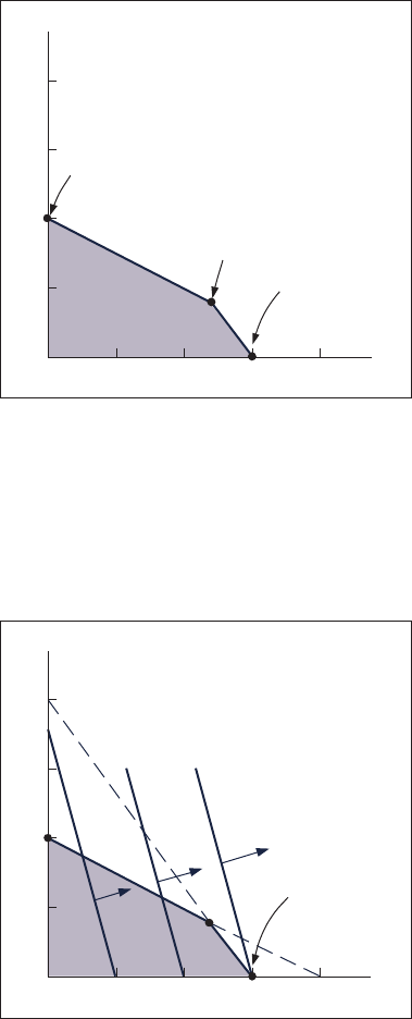
66 Chapter 2 Linear programming: modeL FormuLation and graphiCaL SoLution
moves out of the feasible solution area. Figure 2.12 shows the solution values for all three points,
A, B, and C, and the amount of profit, Z, at each point.
As indicated in the discussion of Figure 2.10, point B is the optimal solution point because
it is the last point the objective function touches before it leaves the solution area. In other
words, the objective function determines which extreme point is optimal. This is because the
objective function designates the profit that will accrue from each combination of
x
1
and
x
2
values at the extreme points. If the objective function had had different coefficients (i.e., dif-
ferent
x
1
and
x
2
profit values), one of the extreme points other than B might have been optimal.
FIGURE 2.13
The optimal
solution with
Z
∙
70x
1
∙
20x
2
10
10
0
x
1
x
2
20 30 40
20
30
40
4x
1
+ 3x
2
= 120
Z = 70x
1
+ 20x
2
x
1
+ 2x
2
= 40
A
B
C
Optimal point:
x
1
= 30 bowls
x
2
= 0 mugs
Z = $2,100
FIGURE 2.12
Solutions at all
corner points
10
10
0
x
x
2
20 30 40
20
30
40
1
A
B
C
x
1
= 0 bowls
x
2
= 20 mugs
Z = $1,000
x
1
= 24 bowls
x
2
= 8 mugs
Z = $1,360
x
1
= 30 bowls
x
2
= 0 mugs
Z = $1,200
Let’s assume for a moment that the profit for a bowl is $70 instead of $40, and the profit for
a mug is $20 instead of $50. These values result in a new objective function,
Z = +70x
1
+ 20x
2
.
If the model constraints for labor or clay are not changed, the feasible solution area remains the
same, as shown in Figure 2.13. However, the location of the objective function in Figure 2.13 is
different from that of the original objective function in Figure 2.10. The reason for this change is
that the new profit coefficients give the linear objective function a new slope.
The slope can be determined by transforming the objective function into the general equation
for a straight line,
y = a + bx,
where y is the dependent variable, a is the y intercept, b is the
slope, and x is the independent variable. For our sample objective function,
x
2
is the dependent
The slope is computed
as the “rise” over
the“run.”
M02_TAYL3045_13_GE_C02.indd 66 26/10/2018 09:08

graphiCaL SoLutionS oF Linear programming modeLS 67
variable corresponding to y (i.e., it is on the vertical axis), and
x
1
is the independent variable.
Thus,the objective function can be transformed into the general equation of a line as follows:
Z = 70x
1
+ 20x
2
20x
2
= Z - 70x
1
x
2
=
Z
20
-
7
2
x
1
c
c
c
y
a
b
This transformation identifies the slope of the new objective function as
-7/2
(the minus sign
indicates that the line slopes downward). In contrast, the slope of the original objective function
was
-4/5.
If we move this new objective function out through the feasible solution area, the last
extremepoint it touches is point C. Simultaneously solving the constraint lines at point C results
in the following solution:
x
1
= 30
4x
1
+ 3x
2
= 120
and
x
2
= 40 - (4x
1
/3)
x
2
= 40 - 4(30)/3
x
2
= 0
Thus, the optimal solution at point C in Figure 2.13 is
x
1
= 30
bowls,
x
2
= 0
mugs, and
Z = +2,100
profit. Altering the objective function coefficients results in a new solution.
This brief example of the effects of altering the objective function highlights two useful
points. First, the optimal extreme point is determined by the objective function, and an extreme
point on one axis of the graph is as likely to be the optimal solution as is an extreme point on a
different axis. Second, the solution is sensitive to the values of the coefficients in the objective
function. If the objective function coefficients are changed, as in our example, the solution may
change. Likewise, if the constraint coefficients are changed, the solution space and solution points
may change also. This information can be of consequence to the decision maker trying to deter-
mine how much of a product to produce. Sensitivity analysis—the use of linear programming to
evaluate the effects of changes in model parameters—is discussed in Chapter 3.
It should be noted that some problems do not have a single extreme point solution. For example,
when the objective function line parallels one of the constraint lines, an entire line segment is bounded
by two adjacent corner points that are optimal; there is no single extreme point on the objective
function line. In this situation, there are multiple optimal solutions. This and other irregular types
of solution outcomes in linear programming are discussed at the end of this chapter.
Slack Variables
Once the optimal solution was found at point B in Figure 2.12, simultaneous equations were
solved to determine the values of
x
1
and
x
2
.
Recall that the solution occurs at an extreme point
where constraint equation lines intersect with each other or with the axis. Thus, the model con-
straints are considered as equations
(= )
rather than
…
or
Ú
inequalities.
There is a standard procedure for transforming
…
inequality constraints into equations. This
transformation is achieved by adding a new variable, called a slack variable, to each constraint.
For the pottery company example, the model constraints are
x
1
+ 2x
2
… 40 hr. of labor
4x
1
+ 3x
2
… 120 lb. of clay
Sensitivity analysis
is used to analyze
changes in model
parameters.
Multiple optimal
solutions can occur
when the objective
function is parallel to
a constraint line.
A slack variable
is added to a
…
constraint to convert
it to an equation
(= ).
A slack variable
represents unused
resources.
M02_TAYL3045_13_GE_C02.indd 67 26/10/2018 09:08
68 Chapter 2 Linear programming: modeL FormuLation and graphiCaL SoLution
The addition of a unique slack variable,
s
1
,
to the labor constraint and
s
2
to the constraint for clay
results in the following equations:
x
1
+ 2x
2
+ s
1
= 40 hr. of labor
4x
1
+ 3x
2
+ s
2
= 120 lb. of clay
The slack variables in these equations,
s
1
and
s
2
,
will take on any value necessary to make the
left-hand side of the equation equal to the right-hand side. For example, consider a hypothetical
solution of
x
1
= 5
and
x
2
= 10.
Substituting these values into the foregoing equations yields
x
1
+ 2x
2
+ s
1
= 40 hr. of labor
5 + 2(10) + s
1
= 40 hr. of labor
s
1
= 15 hr. of labor
and
4x
1
+ 3x
2
+ s
2
= 120 lb. of clay
4(5) + 3(10) + s
2
= 120 lb. of clay
s
2
= 70 lb. of clay
In this example,
x
1
= 5
bowls and
x
2
= 10
mugs represent a solution that does not make
use of the total available amount of labor and clay. In the labor constraint, 5 bowls and 10 mugs
require only 25 hours of labor. This leaves 15 hours that are not used. Thus,
s
1
represents the
amount of unused labor, or slack.
In the clay constraint, 5 bowls and 10 mugs require only 50 pounds of clay. This leaves 70
pounds of clay unused. Thus,
s
2
represents the amount of unused clay. In general, slack variables
represent the amount of unused resources.
The ultimate instance of unused resources occurs at the origin, where
x
1
= 0
and
x
2
= 0.
Substituting these values into the equations yields
x
1
+ 2x
2
+ s
1
= 40
0 + 2(0) + s
1
= 40
s
1
= 40 hr. of labor
and
4x
1
+ 3x
2
+ s
2
= 120
4(0) + 3(0) + s
2
= 120
s
2
= 120 lb. of clay
Because no production takes place at the origin, all the resources are unused; thus, the slack vari-
ables equal the total available amounts of each resource:
s
1
= 40
hours of labor and
s
2
= 120
pounds of clay.
What is the effect of these new slack variables on the objective function? The objective func-
tion for our example represents the profit gained from the production of bowls and mugs,
Z = +40x
1
+ +50x
2
The coefficient $40 is the contribution to profit of each bowl; $50 is the contribution to
profit of each mug. What, then, do the slack variables
s
1
and
s
2
contribute? They contribute
nothing to profit because they represent unused resources. Profit is made only after the resources
are put to use in making bowls and mugs. Using slack variables, we can write the objective
function as
maximize Z = +40x
1
+ +50x
2
+ 0s
1
+ 0s
2
A slack variable
contributes nothing to
the objective function
value.
M02_TAYL3045_13_GE_C02.indd 68 26/10/2018 09:08

graphiCaL SoLutionS oF Linear programming modeLS 69
As in the case of decision variables (
x
1
and
x
2
), slack variables can have only nonnega-
tive values because negative resources are not possible. Therefore, for this model formulation,
x
1
, x
2
, s
1
,
and
s
2
Ú 0.
The complete linear programming model can be written in what is referred to as standard
form with slack variables as follows:
maximize Z = +40x
1
+ +50x
2
+ 0s
1
+ 0s
2
subject to
x
1
+ 2x
2
+ s
1
= 40
4x
1
+ 3x
2
+ s
2
= 120
x
1
, x
2
, s
1
, s
2
Ú 0
The solution values, including the slack at each solution point, are summarized as follows:
FIGURE 2.14
Solutions at
points A, B, and C
with slack
10
10
0
x
1
x
2
20 30 40
20
30
40
A
B
C
4x
1
+ 3x
2
+ s
2
= 120
x
1
+ 2x
2
+
s
1
= 40
x
1
= 0
x
2
= 20
s
1
= 0
s
2
= 60
x
1
= 24
x
2
= 8
s
1
= 0
s
2
= 0
x
1
= 30
x
2
= 0
s
1
= 10
s
2
= 0
Solution Summary with Slack
Point Solution Values Z Slack
A
x
1
= 0 bowls, x
2
= 20 mugs
$1,000
s
1
= 0 hr.; s
2
= 60 lb.
B
x
1
= 24 bowls, x
2
= 8 mugs
$1,360
s
1
= 0 hr.; s
2
= 0 lb.
C
x
1
= 30 bowls, x
2
= 0 mugs
$1,200
s
1
= 10 hr.; s
2
= 0 lb.
Figure 2.14 shows the graphical solution of this example, with slack variables included at
each solution point.
Summary of the Graphical Solution Steps
The steps for solving a graphical linear programming model are summarized here:
1. Plot the model constraints as equations on the graph; then, considering the inequalities of
the constraints, indicate the feasible solution area.
2. Plot the objective function; then, move this line out from the origin to locate the optimal
solution point.
3. Solve simultaneous equations at the solution point to find the optimal solution values.
M02_TAYL3045_13_GE_C02.indd 69 26/10/2018 09:08

70 Chapter 2 Linear programming: modeL FormuLation and graphiCaL SoLution
Or
1. Solve simultaneous equations at each corner point to find the solution values at each point.
2. Substitute these values into the objective function to find the set of values that results in the
maximum Z value.
A Minimization Model Example
As mentioned at the beginning of this chapter, there are two types of linear programming prob-
lems: maximization problems (like the Beaver Creek Pottery Company example) and minimiza-
tion problems. A minimization problem is formulated the same basic way as a maximization
problem, except for a few minor differences. The following sample problem will demonstrate the
formulation of a minimization model.
A farmer is preparing to plant a crop in the spring and needs to fertilize a field. There are
two brands of fertilizer to choose from, Super-gro and Crop-quick. Each brand yields a specific
amount of nitrogen and phosphate per bag, as follows:
Management Science Application
Renewable Energy Investment Decisions at GE Energy
g
eneral Electric Energy is the world’s second-largest manu-
facturer of wind turbines and has a growing solar busi-
ness, and GE Capitals’ Energy Financial Services invests
billions of dollars each year in renewable energy power plants.
To help it make investment decisions GE Energy developed a
mathematical programming model to project the financial
performance of its renewable energy plants and forecast new
renewable energy capacity and generation over a 10-year hori-
zon. Building renewable energy power plants is more expensive
than building conventional plants, so their construction is driven
by government incentives and mandates called renewable port-
folio standards (RPS), which require utilities to meet a percentage
of demand with renewable energy sources. Utilities that cannot
meet these mandates either purchase renewable energy credits
from utilities that have excess renewable energy or pay a compli-
ance payment. The model’s objective function minimizes the cost
of meeting the RPS mandates over a 10-year horizon (which is
equal to the cost of producing energy at new plants plus energy
transportation costs plus penalties paid for noncompliance), sub-
ject to constraints for meeting RPS demand by program and year,
meeting transmission capacity constraints, new building capacity
constraints, and meeting energy capacity constraints. Decision
variables include (for the time horizon) renewable energy plants
built by technology, resource, and year; renewable energy trans-
ported across states by year; and penalties paid to states for not
meeting RPS mandates by year. Since it was implemented, the
model has helped GE estimate renewable energy credit prices
used in renewable project evaluations, forecast renewable energy
demand, evaluate the effectiveness of government policies, and
advocate for effective policies.
Source: Based on S. Bollapragada, B. Owens, and S. Taub, “Practice
Summaries: An Optimization Model to Support Renewable Energy
Investment Decisions,” Interfaces 41, no. 4 (July–August 2011): 394–95.
Michele Tantussi/Getty Images
Chemical Contribution
Brand Nitrogen (lb./bag) Phosphate (lb./bag)
Super-gro 2 4
Crop-quick 4 3
M02_TAYL3045_13_GE_C02.indd 70 26/10/2018 09:08

a minimization modeL exampLe 71
The farmer’s field requires at least 16 pounds of nitrogen and at least 24 pounds of phosphate.
Super-gro costs $6 per bag, and Crop-quick costs $3. The farmer wants to know how many bags
of each brand to purchase to minimize the total cost of fertilizing. This scenario is illustrated in
Figure 2.15.
FIGURE 2.15
Fertilizing
farmer’s field
Nitrogen
2 lb.
Phosphate
4 lb.
Super-gro
$6
Nitrogen
4 lb.
Phosphate
3 lb.
Crop-quick
$3
Requirements
$16 lb. nitrogen
$24 lb. phosphate
The steps in the linear programming model formulation process are summarized as follows:
Summary of LP Model Formulation Steps
Step 1: Define the decision variables
How many bags of Super-gro and Crop-quick to buy
Step 2: Define the objective function
Minimize cost
Step 3: Define the constraints
The field requirements for nitrogen and phosphate
Decision Variables
This problem contains two decision variables, representing the number of bags of each brand of
fertilizer to purchase:
x
1
= bags of Super@gro
x
2
= bags of Crop@quick
M02_TAYL3045_13_GE_C02.indd 71 26/10/2018 09:08
72 Chapter 2 Linear programming: modeL FormuLation and graphiCaL SoLution
The Objective Function
The farmer’s objective is to minimize the total cost of fertilizing. The total cost is the sum of the
individual costs of each type of fertilizer purchased. The objective function that represents total
cost is expressed as
minimize Z = +6x
1
+ 3x
2
where
+6x
1
= cost of bags of Super@gro
+3x
2
= cost of bags of Crop@quick
Model Constraints
The requirements for nitrogen and phosphate represent the constraints of the model. Each bag of
fertilizer contributes a number of pounds of nitrogen and phosphate to the field. The constraint
for nitrogen is
2x
1
+ 4x
2
Ú 16 lb.
where
2x
1
= the nitrogen contribution (lb.) per bag of Super@gro
4x
2
= the nitrogen contribution (lb.) per bag of Crop@quick
Rather than a
…
(less than or equal to) inequality, as used in the Beaver Creek Pottery Com-
pany model, this constraint requires a
Ú
(greater than or equal to) inequality. This is because
the nitrogen content for the field is a minimum requirement specifying that at least 16 pounds
of nitrogen be deposited on the farmer’s field. If a minimum cost solution results in more than
16 pounds of nitrogen on the field, that is acceptable; however, the amount cannot be less than
16 pounds.
The constraint for phosphate is constructed like the constraint for nitrogen:
4x
1
+ 3x
2
Ú 24 lb.
With this example, we have shown two of the three types of linear programming model con-
straints,
…
and
Ú .
The third type is an exact equality,
= .
This type specifies that a constraint
requirement must be exact. For example, if the farmer had said that the phosphate requirement
for the field was exactly 24 pounds, the constraint would have been
4x
1
+ 3x
2
= 24 lb.
As in our maximization model, there are also nonnegativity constraints in this problem to
indicate that negative bags of fertilizer cannot be purchased:
x
1
, x
2
Ú 0
The complete model formulation for this minimization problem is
minimize Z = +6x
1
+ 3x
2
subject to
2x
1
+ 4x
2
Ú 16 lb of nitrogen
4x
1
+ 3x
2
Ú 24 lb of phosphate
x
1
, x
2
Ú 0
The three types of
linear programming
constraints are
… , = ,
and
Ú .
M02_TAYL3045_13_GE_C02.indd 72 26/10/2018 09:08

a minimization modeL exampLe 73
Graphical Solution of a Minimization Model
We follow the same basic steps in the graphical solution of a minimization model as in a maxi-
mization model. The fertilizer example will be used to demonstrate the graphical solution of a
minimization model.
The first step is to graph the equations of the two model constraints, as shown in Figure 2.16.
Next, the feasible solution area is chosen, to reflect the
Ú
inequalities in the constraints, as
shown in Figure 2.17.
FIGURE 2.16
Constraint lines
for fertilizer
model
2
2
0
x
1
x
2
4 6 8 10 12 14
4
6
8
10
12
14
4x
1
+ 3x
2
= 24
2x
1
+ 4x
2
= 16
FIGURE 2.17
Feasible solution
area
2
2
0
x
1
x
2
4 6 8 10 12 14
4
6
8
10
12
14
Feasible
solution
area
After the feasible solution area has been determined, the second step in the graphical solution
approach is to locate the optimal point. Recall that in a maximization problem, the optimal solu-
tion is on the boundary of the feasible solution area that contains the point(s) farthest from the
origin. The optimal solution point in a minimization problem is also on the boundary of the fea-
sible solution area; however, the boundary contains the point(s) closest to the origin (zero being
the lowest cost possible).
As in a maximization problem, the optimal solution is located at one of the extreme points of
the boundary. In this case, the corner points represent extremities in the boundary of the feasible
In a minimization
problem the boundary
of the feasible
solution area closest
to the origin contains
the optimal extreme
point.
M02_TAYL3045_13_GE_C02.indd 73 26/10/2018 09:08

74 Chapter 2 Linear programming: modeL FormuLation and graphiCaL SoLution
solution area that are closest to the origin. Figure 2.18 shows the three corner points—A, B, and
C—and the objective function line.
As the objective function edges toward the origin, the last point it touches in the feasible
solution area is A. In other words, point A is the closest the objective function can get to the
origin without encompassing infeasible points. Thus, it corresponds to the lowest cost that can
be attained.
FIGURE 2.18
The optimal
solution point
2
2
0
x
1
x
2
4 6 8 10 12 14
4
6
8
10
12
14
Z = 6x
1
+ 3x
2
x
1
= 0 bags of Super-gro
x
2
= 8 bags of Crop-quick
Z = $24
A
B
C
Management Science Application
Determining Optimal Fertilizer Mixes at Soquimich (South America)
S
oquimich, a Chilean fertilizer manufacturer, is the lead-
ing producer and distributor of specialty fertilizers in the
world, with revenues of almost US$0.5 billion in more than
80 countries. Soquimich produces four main specialty fertilizers
and more than 200 fertilizer blends, depending on the needs
of its customers. Farmers want the company to quickly recom-
mend optimal fertilizer blends that will provide the appropriate
quantity of ingredients for their particular crop at the lowest
possible cost. A farmer will provide a company sales representa-
tive with information about previous crop yields and his or her
target yields, and then company representatives will visit the
farm to obtain soil samples, which are analyzed in the company
labs. A report is generated, which indicates the soil require-
ments for nutrients, including nitrogen, phosphorus, potassium,
boron, magnesium, sulfur, and zinc. Given these soil require-
ments, company experts determine an optimal fertilizer blend,
using a linear programming model that includes constraints
for the nutrient quantities required by the soil (for a particu-
lar crop) and an objective function that minimizes production
costs. Previously the company determined fertilizer blend rec-
ommendations by using a time-consuming manual procedure
conducted by experts. The linear programming model enables
the company to provide accurate, quick, low-cost (discounted)
estimates to its customers, which has helped the company gain
new customers and increase its market share.
Source: Based on A. M. Angel, L. A. Taladriz, and R. Weber, “Soquimich
Uses a System Based on Mixed-Integer Linear Programming and
Expert Systems to Improve Customer Service,” Interfaces 33, no. 4
(July–August 2003): 41–52.
Alex Havret/Dk Images
M02_TAYL3045_13_GE_C02.indd 74 26/10/2018 09:08
a minimization modeL exampLe 75
The final step in the graphical solution approach is to solve for the values of
x
1
and
x
2
at point
A. Because point A is on the
x
2
axis,
x
1
= 0;
thus,
4(0) + 3x
2
= 24
x
2
= 8
Given that the optimal solution is
x
1
= 0, x
2
= 8,
the minimum cost, Z, is
Z = +6x
1
+ +3x
2
Z = 6(0) + 3(8)
= +24
This means the farmer should not purchase any Super-gro but, instead, should purchase eight bags
of Crop-quick, at a total cost of $24.
Surplus Variables
Greater-than or equal-to constraints cannot be converted to equations by adding slack variables,
as with
…
constraints. Recall our fertilizer model, formulated as
minimize Z = +6x
1
+ +3x
2
subject to
2x
1
+ 4x
2
Ú 16 lb. of nitrogen
4x
1
+ 3x
2
Ú 24 lb. of phosphate
x
1
, x
2
Ú 0
where
x
1
= bags of Super@gro fertilizer
x
2
= bags of Crop@quick fertilizer
Z = farmers total cost (+) of purchasing fertilizer
Because this problem has
Ú
constraints as opposed to the
…
constraints of the Beaver
Creek Pottery Company maximization example, the constraints are converted to equations a little
differently.
Instead of adding a slack variable as we did with a
Ú
constraint, we subtract a surplus
variable. Whereas a slack variable is added and reflects unused resources, a surplus variable is
subtracted and reflects the excess above a minimum resource requirement level. Like a slack
variable, a surplus variable is represented symbolically by
s
1
and must be nonnegative.
For the nitrogen constraint, the subtraction of a surplus variable gives
2x
1
+ 4x
2
- s
1
= 16
The surplus variable
s
1
transforms the nitrogen constraint into an equation.
As an example, consider the hypothetical solution
x
1
= 0
x
2
= 10
Substituting these values into the previous equation yields
2(0) + 4(10) - s
1
= 16
-s
1
= 16 - 40
s
1
= 24 lb. of nitrogen
In this equation,
s
1
can be interpreted as the extra amount of nitrogen above the minimum
requirement of 16 pounds that would be obtained by purchasing 10 bags of Crop-quick fertilizer.
A surplus variable is
subtracted from a
Ú
constraint to convert
it to an equation
(= ).
A surplus variable
represents an excess
above a constraint
requirement level.
M02_TAYL3045_13_GE_C02.indd 75 26/10/2018 09:08

76 Chapter 2 Linear programming: modeL FormuLation and graphiCaL SoLution
In a similar manner, the constraint for phosphate is converted to an equation by subtracting
a surplus variable,
s
2
:
4x
1
+ 3x
2
- s
2
= 24
As is the case with slack variables, surplus variables contribute nothing to the overall cost
of a model. For example, putting additional nitrogen or phosphate on the field will not affect the
farmer’s cost; the only thing affecting cost is the number of bags of fertilizer purchased. As such,
the standard form of this linear programming model is summarized as
minimize Z = +6x
1
+ 3x
2
+ 0s
1
+ 0s
2
subject to
2x
1
+ 4x
2
- s
1
= 16
4x
1
+ 3x
2
- s
2
= 24
x
1
, x
2
, s
1
, s
2
Ú 0
Figure 2.19 shows the graphical solutions for our example, with surplus variables included
at each solution point.
FIGURE 2.19
Graph of the
fertilizer example
2
4
6
8
10
12
2
0
4 6 8 10 12
x
1
x
2
A
B
C
x
1
= 0
x
2
= 8
s
1
= 16
s
2
= 0
Z
= 24
x
1
= 4.8
x
2
= 1.6
s
1
= 0
s
2
= 0
Z = 33.6
x
1
= 8
x
2
= 0
s
1
= 0
s
2
= 8
Z = 48
Irregular Types of Linear Programming Problems
The basic forms of typical maximization and minimization problems have been shown in this
chapter. However, there are several special types of atypical linear programming problems.
Although these special cases do not occur frequently, they will be described so that you can rec-
ognize them when they arise. These special types include problems with more than one optimal
solution, infeasible problems, and problems with unbounded solutions.
Multiple Optimal Solutions
Consider the Beaver Creek Pottery Company example, with the objective function changed from
Z = 40x
1
+ 50x
2
to
Z = 40x
1
+ 30x
2
:
For some linear
programming models,
the general rules do
not always apply.
M02_TAYL3045_13_GE_C02.indd 76 26/10/2018 09:08

irreguLar typeS oF Linear programming probLemS 77
maximize Z = 40x
1
+ 30x
2
subject to
x
1
+ 2x
2
… 40 hr. of labor
4x
1
+ 3x
2
… 120 lb. of clay
x
1
, x
2
Ú 0
where
x
1
= bowls produced
x
2
= mugs produced
The graph of this model is shown in Figure 2.20. The slight change in the objective function
makes it now parallel to the constraint line,
4x
1
+ 3x
2
= 120.
Both lines now have the same slope
of
-4/3.
Therefore, as the objective function edge moves outward from the origin, it touches the
whole line segment BC rather than a single extreme corner point before it leaves the feasible solu-
tion area. This means that every point along this line segment is optimal (i.e., each point results
in the same profit of
Z = +1,200
). The endpoints of this line segment, B and C, are typically
referred to as the alternate optimal solutions. It is understood that these points represent the
endpoints of a range of optimal solutions.
Alternate optimal
solutions are at
the endpoints of
the constraint line
segment that the
objective function
parallels.
FIGURE 2.20
Graph of the
Beaver Creek
Pottery Company
example with
multiple optimal
solutions
C
B
A
Point B
x
1
= 24
x
2
= 8
Z = 1,200
Point C
x
1
= 30
x
2
= 0
Z = 1,200
10
10
0
x
1
x
2
20 30 40
20
30
40
The pottery company, therefore, has several options in deciding on the number of bowls and
mugs to produce. Multiple optimal solutions can benefit the decision maker because the number
of decision options is enlarged. The multiple optimal solutions (along the line segment BC in
Figure 2.20) allow the decision maker greater flexibility. For example, in the case of Beaver Creek
Pottery Company, it may be easier to sell bowls than mugs; thus, the solution at point C, where
only bowls are produced, would be more desirable than the solution at point B, where a mix of
bowls and mugs is produced.
An Infeasible Problem
In some cases, a linear programming problem has no feasible solution area; thus, there is no
solution to the problem. An example of an infeasible problem is formulated next and depicted
graphically in Figure 2.21:
maximize Z = 5x
1
+ 3x
2
subject to
4x
1
+ 2x
2
… 8
x
1
Ú 4
x
2
Ú 6
x
1
, x
2
Ú 0
Multiple optimal
solutions provide
greater flexibility to
the decision maker.
An infeasible problem
has no feasible
solution area; every
possible solution
point violates one or
more constraints.
M02_TAYL3045_13_GE_C02.indd 77 26/10/2018 09:08

78 Chapter 2 Linear programming: modeL FormuLation and graphiCaL SoLution
Point A in Figure 2.21 satisfies only the constraint
4x
1
+ 2x
2
… 8,
whereas point C satis-
fies only the constraints
x
1
Ú 4
and
x
2
Ú 6.
Point B satisfies none of the constraints. The three
constraints do not overlap to form a feasible solution area. Because no point satisfies all three
constraints simultaneously, there is no solution to the problem. Infeasible problems do not typi-
cally occur, but when they do, they are usually a result of errors in defining the problem or in
formulating the linear programming model.
FIGURE 2.21
Graph of an
infeasible
problem
2
4
6
8
10
12
2
0
4 6 8 10 12
x
1
x
2
B
C
A
x
1
= 4
x
2
= 6
4x
1
+ 2x
2
= 8
An Unbounded Problem
In some problems, the feasible solution area formed by the model constraints is not closed. In
these cases, it is possible for the objective function to increase indefinitely without ever reaching
a maximum value because it never reaches the boundary of the feasible solution area.
An example of this type of unbounded problem is formulated next and shown graphically
in Figure 2.22:
maximize Z = 4x
1
+ 2x
2
subject to
x
1
Ú 4
x
2
… 2
x
1
, x
2
Ú 0
In an unbounded
problem the objective
function can increase
indefinitely without
reaching a maximum
value.
FIGURE 2.22
An unbounded
problem
2
4
6
8
10
12
2
0
4 6 8 10 12
x
1
x
2
Z = 4x
1
+ 2
x
2
M02_TAYL3045_13_GE_C02.indd 78 26/10/2018 09:08
CharaCteriStiCS oF Linear programming probLemS 79
In Figure 2.22, the objective function is shown to increase without bound; thus, a solution is never
reached.
Unlimited profits are not possible in the real world; an unbounded solution, like an infeasible
solution, typically reflects an error in defining the problem or in formulating the model.
Characteristics of Linear Programming Problems
Now that we have had the opportunity to construct several linear programming models, let’s
review the characteristics that identify a linear programming problem.
A linear programming problem requires a choice between alternative courses of action (i.e.,
a decision). The decision is represented in the model by decision variables. A typical choice task
for a business firm is deciding how much of several different products to produce, as in the Beaver
Creek Pottery Company example presented earlier in this chapter. Identifying the choice task and
defining the decision variables is usually the first step in the formulation process because it is quite
difficult to construct the objective function and constraints without first identifying the decision
variables.
The problem encompasses an objective that the decision maker wants to achieve. The two
most frequently encountered objectives for a business are maximizing profit and minimizing
cost.
A third characteristic of a linear programming problem is that restrictions exist, making
unlimited achievement of the objective function impossible. In a business firm, these restrictions
often take the form of limited resources, such as labor or material; however, the sample models
in this chapter exhibit a variety of problem restrictions. These restrictions, as well as the objec-
tive, must be definable by mathematical functional relationships that are linear. Defining these
relationships is typically the most difficult part of the formulation process.
Properties of Linear Programming Models
In addition to encompassing only linear relationships, a linear programming model also has several
other implicit properties, which have been exhibited consistently throughout the examples in this
chapter. The term linear not only means that the functions in the models are graphed as a straight
line; it also means that the relationships exhibit proportionality. In other words, the rate of
change, or slope, of the function is constant; therefore, changes of a given size in the value of a
decision variable will result in exactly the same relative changes in the functional value.
Linear programming also requires that the objective function terms and the constraint terms be
additive. For example, in the Beaver Creek Pottery Company model, the total profit (Z) must equal
the sum of profits earned from making bowls
(+40x
1
)
and mugs
(+50x
2
).
Also, the total resources
used must equal the sum of the resources used for each activity in a constraint (e.g., labor).
Another property of linear programming models is that the solution values (of the decision
variables) cannot be restricted to integer values; the decision variables can take on any frac-
tional value. Thus, the variables are said to be continuous or divisible, as opposed to integer or
discrete. For example, although decision variables representing bowls or mugs or airplanes or
automobiles should realistically have integer (whole number) solutions, the solution methods
for linear programming will not necessarily provide such solutions. This is a property that will
be discussed further as solution methods are presented in subsequent chapters.
The final property of linear programming models is that the values of all the model param-
eters are assumed to be constant and known with certainty. In real situations, however, model
parameters are frequently uncertain because they reflect the future as well as the present, and
future conditions are rarely known with certainty.
To summarize, a linear programming model has the following general properties: linear-
ity, proportionality, additivity, divisibility, and certainty. As various linear programming solution
methods are presented throughout this book, these properties will become more obvious, and their
impact on problem solution will be discussed in greater detail.
The solution space
isnot completely
closed in.
The components of a
linear programming
model are an
objective function,
decision variables,
and constraints.
Proportionality
means the slope
of a constraint or
objective function line
is constant.
The terms in the
objective function
or constraints are
additive.
The values of
decision variables
are continuous or
divisible.
All model
parametersare
assumed to be known
with certainty.
M02_TAYL3045_13_GE_C02.indd 79 26/10/2018 09:08

80 Chapter 2 Linear programming: modeL FormuLation and graphiCaL SoLution
Summary
The two example problems in this chapter were formulated as linear programming models to
demonstrate the modeling process. These problems were similar in that they concerned achiev-
ing some objective subject to a set of restrictions or requirements. Linear programming models
exhibit certain common characteristics:
● An objective function to be maximized or minimized
● A set of constraints
● Decision variables for measuring the level of activity
● Linearity among all constraint relationships and the objective function
The graphical approach to the solution of linear programming problems is not a very efficient
means of solving problems. For one thing, drawing accurate graphs is tedious. Moreover, the
graphical approach is limited to models with only two decision variables. However, the analysis
of the graphical approach provides valuable insight into linear programming problems and their
solutions.
In the graphical approach, once the feasible solution area and the optimal solution point have
been determined from the graph, simultaneous equations are solved to determine the values of
x
1
and
x
2
at the solution point.In Chapter 3 we will show how linear programming solutions can be
obtained using computer programs.
As a prelude to the problems, this section presents example solutions to two linear programming
problems.
Problem Statement
Moore’s Meatpacking Company produces a hot dog mixture in 1,000-pound batches. The mixture
contains two ingredients—chicken and beef. The cost per pound of each of these ingredients is
as follows:
Ingredient Cost/lb.
Chicken $3
Beef $5
Each batch has the following recipe requirements:
a. At least 500 pounds of chicken
b. At least 200 pounds of beef
The ratio of chicken to beef must be at least 2 to 1. The company wants to know the optimal
mixture of ingredients that will minimize cost. Formulate a linear programming model for this
problem.
Solution
Step 1: Identify Decision Variables
Recall that the problem should not be “swallowed whole.” Identify each part of the model sepa-
rately, starting with the decision variables:
x
1
= lb. of chicken
x
2
= lb. of beef
Example Problem
Solutions
M02_TAYL3045_13_GE_C02.indd 80 26/10/2018 09:08

exampLe probLem SoLutionS 81
Step 2: Formulate the Objective Function
minimize Z = +3x
1
+ +5x
2
where
Z = cost per1,000@lb batch
+3x
1
= cost of chicken
+5x
2
= cost of beef
Step 3: Establish Model Constraints
The constraints of this problem are embodied in the recipe restrictions and (not to be overlooked)
the fact that each batch must consist of 1,000 pounds of mixture:
x
1
+ x
2
= 1,000 lb.
x
1
Ú 500 lb. of chicken
x
2
Ú 200 lb. of beef
x
1
/x
2
Ú 2/1 or x
1
- 2x
2
Ú 0
and
x
1
, x
2
Ú 0
The Model
minimize Z = +3x
1
+ +5x
2
subject to
x
1
+ x
2
= 1,000
x
1
Ú 500
x
2
Ú 200
x
1
- 2x
2
Ú 0
x
1
, x
2
Ú 0
Problem Statement
Solve the following linear programming model graphically:
maximize Z = 4x
1
+ 5x
2
subject to
x
1
+ 2x
2
… 10
6x
1
+ 6x
2
… 36
x
1
… 4
x
1
, x
2
Ú 0
M02_TAYL3045_13_GE_C02.indd 81 26/10/2018 09:08

82 Chapter 2 Linear programming: modeL FormuLation and graphiCaL SoLution
The feasible
solution space
and extreme
points
x
1
10
2
2
0
x
2
4 6 8 10
4
6
8
A
B
C
D
x
1
10
2
2
0
x
2
4 6 8 10
4
6
8
x
1
= 4
6x
1
+ 6x
2
= 36
x
1
+ 2x
2
= 10
The constraint
equations
Solution
Step 1: Plot the Constraint Lines as Equations
A simple method for plotting constraint lines is to set one of the constraint variables equal to zero
and solve for the other variable to establish a point on one of the axes. The three constraint lines
are graphed in the following figure:
Step 2: Determine the Feasible Solution Area
The feasible solution area is determined by identifying the space that jointly satisfies the
…
conditions of all three constraints, as shown in the following figure:
M02_TAYL3045_13_GE_C02.indd 82 26/10/2018 09:08

exampLe probLem SoLutionS 83
Step 3: Determine the Solution Points
The solution at point A can be determined by noting that the constraint line intersects the
x
2
axis at
5; thus,
x
2
= 5, x
1
= 0,
and
Z = 25.
The solution at point D on the other axis can be determined
similarly; the constraint intersects the axis at
x
1
= 4, x
2
= 0,
and
Z = 16.
The values at points B and C must be found by solving simultaneous equations. Note that
point B is formed by the intersection of the lines
x
1
+ 2x
2
= 10
and
6x
1
+ 6x
2
= 36.
First,
convert both of these equations to functions of
x
1
:
x
1
+ 2x
2
= 10
x
1
= 10 - 2x
2
and
6x
1
+ 6x
2
= 36
6x
1
= 36 - 6x
2
x
1
= 6 - x
2
Now, set the equations equal and solve for
x
2
:
10 - 2x
2
= 6 - x
2
-x
2
= -4
x
2
= 4
Substituting
x
2
= 4
into either of the two equations gives a value for
x
1
:
x
1
= 6 - x
2
x
1
= 6 - (4)
x
1
= 2
Thus, at point B,
x
1
= 2, x
2
= 4,
and
Z = 28.
At point C,
x
1
= 4.
Substituting
x
1
= 4
into the equation
x
1
= 6 - x
2
gives a value for
x
2
:
4 = 6 - x
2
x
2
= 2
Thus,
x
1
= 4, x
2
= 2,
and
Z = 26.
Step 4: Determine the Optimal Solution
The optimal solution is at point B, where
x
1
= 2, x
2
= 4,
and
Z = 28.
The optimal solution and
solutions at the other extreme points are summarized in the following figure:
Optimal solution
point
x
1
10
2
2
0
x
2
4 6 8 10
4
6
8
A
B
C
D
x
1
= 0
x
2
= 5
Z = 25
Optimal
x
1
= 2
x
2
= 4
Z = 28
x
1
= 4
x
2
= 2
Z = 26
x
1
= 4
x
2
= 0
Z = 16
M02_TAYL3045_13_GE_C02.indd 83 26/10/2018 09:08

84 Chapter 2 Linear programming: modeL FormuLation and graphiCaL SoLution
Problems
1. In Problem 40 in Chapter 1, when Tracy McCoy wakes up Saturday morning, she remembers
that she promised the PTA she would make some cakes and/or homemade bread for its bake sale
that afternoon. However, she does not have time to go to the store to get ingredients, and she has
only a short time to bake things in her oven. Because cakes and breads require different baking
temperatures, she cannot bake them simultaneously, and she has only 3 hours available to bake.
A cake requires 3 cups of flour, and a loaf of bread requires 8 cups; Tracy has 20 cups of flour.
A cake requires 45 minutes to bake, and a loaf of bread requires 30 minutes. The PTA will sell
a cake for $10 and a loaf of bread for $6. Tracy wants to decide how many cakes and loaves of
bread she should make.
a. Formulate a linear programming model for this problem.
b. Solve this model by using graphical analysis.
2. The Munchies Cereal Company makes a cereal from several ingredients. Two of the ingredients,
oats and rice, provide vitamins A and B. The company wants to know how many ounces of oats and
rice it should include in each box of cereal to meet the minimum requirements of 48 milligrams of
vitamin A and 12 milligrams of vitamin B while minimizing cost. An ounce of oats contributes 8
milligrams of vitamin A and 1 milligram of vitamin B, whereas an ounce of rice contributes 6 mil-
ligrams of A and 2 milligrams of B. An ounce of oats costs $0.05, and an ounce of rice costs $0.03.
a. Formulate a linear programming model for this problem.
b. Solve this model by using graphical analysis.
3. What would be the effect on the optimal solution in Problem 2 if the cost of rice increased from
$0.03 per ounce to $0.06 per ounce?
4. The Kalo Fertilizer Company makes a fertilizer using two chemicals that provide nitrogen, phos-
phate, and potassium. A pound of ingredient 1 contributes 10 ounces of nitrogen and 6 ounces
of phosphate, whereas a pound of ingredient 2 contributes 2 ounces of nitrogen, 6 ounces of
phosphate, and 1 ounce of potassium. Ingredient 1 costs $3 per pound, and ingredient 2 costs $5
per pound. The company wants to know how many pounds of each chemical ingredient to put
into a bag of fertilizer to meet the minimum requirements of 20 ounces of nitrogen, 36 ounces of
phosphate, and 2 ounces of potassium while minimizing cost.
a. Formulate a linear programming model for this problem.
b. Solve this model by using graphical analysis.
5. A metal shop fabricates windows and doors to construction companies. To fabricate these, the
shop uses iron, glass, and labor. The company has 80 units of standard size iron, 60 square feet of
glass, and unlimited hours of labor but the shop has to use 50 hours of labor. The following table
shows the requirement of these resources to produce one window and one door.
Product Window (x1) Doors (x2)
Iron 3 4
Glass 7 2
Labor 3 4
Cost € 500 € 400
The metal shop wants to determine the number of windows and doors it needs to fabricate to
minimize its cost. Assume that fractional values of windows and doors are acceptable.
a. Formulate a linear programming model for this problem.
b. Solve this model by using graphical analysis.
6. Refer to Problem 5.
a. How much iron and labor will be unused if the optimal number of windows and doors are produced?
b. Explain the effect on the optimal solution of changing the profit on a window from € 500
to € 300.
M02_TAYL3045_13_GE_C02.indd 84 26/10/2018 09:08
probLemS 85
7. The Crumb and Custard Bakery makes coffee cakes and Danish pastries in large pans. The main
ingredients are flour and sugar. There are 25 pounds of flour and 16 pounds of sugar available, and
the demand for coffee cakes is 5. Five pounds of flour and 2 pounds of sugar are required to make
a pan of coffee cakes, and 5 pounds of flour and 4 pounds of sugar are required to make a pan of
Danish. A pan of coffee cakes has a profit of $1, and a pan of Danish has a profit of $5. Determine
the number of pans of cakes and Danish to produce each day so that profit will be maximized.
a. Formulate a linear programming model for this problem.
b. Solve this model by using graphical analysis.
8. In Problem 7, how much flour and sugar will be left unused if the optimal numbers of cakes and
Danish are baked?
9. Solve the following linear programming model graphically:
maximize Z = 3x
1
+ 6x
2
subject to
3x
1
+ 2x
2
… 18
x
1
+ x
2
Ú 5
x
1
… 4
x
1
, x
2
Ú 0
10. The Elixer Drug Company produces a drug from two ingredients. Each ingredient contains the
same three antibiotics, in different proportions. One gram of ingredient 1 contributes 3 units, and
1 gram of ingredient 2 contributes 1 unit of antibiotic 1; the drug requires 6 units. At least 4 units
of antibiotic 2 are required, and the ingredients contribute 1 unit each per gram. At least 12 units
of antibiotic 3 are required; a gram of ingredient 1 contributes 2 units, and a gram of ingredient 2
contributes 6 units. The cost for a gram of ingredient 1 is $80, and the cost for a gram of ingredient
2 is $50. The company wants to formulate a linear programming model to determine the number
of grams of each ingredient that must go into the drug to meet the antibiotic requirements at the
minimum cost.
a. Formulate a linear programming model for this problem.
b. Solve this model by using graphical analysis.
11. A jewelry store makes necklaces and bracelets from gold and platinum. The store has 18 ounces
of gold and 20 ounces of platinum. Each necklace requires 3 ounces of gold and 2 ounces of
platinum, whereas each bracelet requires 2 ounces of gold and 4 ounces of platinum. The demand
for bracelets is no more than four. A necklace earns $300 in profit and a bracelet, $400. The store
wants to determine the number of necklaces and bracelets to make to maximize profit.
a. Formulate a linear programming model for this problem.
b. Solve this model by using graphical analysis.
12. In Problem 11, explain the effect on the optimal solution of increasing the profit on a bracelet
from $400 to $600. What will be the effect of changing the platinum requirement for a necklace
from 2 ounces to 3 ounces?
13. In Problem 11:
a. The maximum demand for bracelets is 4. If the store produces the optimal number of bracelets
and necklaces, will the maximum demand for bracelets be met? If not, by how much will it
be missed?
b. What profit for a necklace would result in no bracelets being produced, and what would be
the optimal solution for this profit?
14. A clothier makes coats and slacks. The two resources required are wool cloth and labor. The
clothier has 150 square yards of wool and 200 hours of labor available. Each coat requires 3 square
yards of wool and 10 hours of labor, whereas each pair of slacks requires 5 square yards of wool
M02_TAYL3045_13_GE_C02.indd 85 26/10/2018 09:08
86 Chapter 2 Linear programming: modeL FormuLation and graphiCaL SoLution
and 4 hours of labor. The profit for a coat is $50, and the profit for slacks is $40. The clothier wants
to determine the number of coats and pairs of slacks to make so that profit will be maximized.
a. Formulate a linear programming model for this problem.
b. Solve this model by using graphical analysis.
15. In Problem 14, what would be the effect on the optimal solution if the available labor were
increased from 200 to 240 hours?
16. Amelia wants to do a part time job during her spring break. She has two jobs now—one in an
admissions office and the other in a nearby restaurant. She does not want to work for more than
40 hours per week. She believes that working in the restaurant is easier than working in the admis-
sions office. Since the job at the admissions office demands a high degree of attention, she wants
to work more in the restaurant. For every 1 hour of working at the admissions office, she plans to
work 2 hours in the restaurant. She wants to work up to 22 hours in the restaurant. She will get
a revenue of £9 per hour of work at the admissions office and £7 per hour in the restaurant. She
wants to determine the number of hours she should work in the admissions office (x
1
) and the
restaurant (x
2
) to maximize her earning per week during the spring break.
a. Formulate a linear programming model for this problem.
b. Solve this model by using graphical analysis.
17. In Problem 16:
a. If Amelia works 35 hours weekly, will she make more money?
b. If the admissions office reduces Amelia’s wage to £8 per hour, and restaurant raises the wage
to £9 per hour, and Amelia works up to 25 hours at the restaurant, will these changes affect
her revenue?
c. Alternatively, if she plans to work for 50 hours per week, will this affect her revenue?
d. If Amelia combines alternatives proposed in b and c, will this affect her profit?
18. Solve the following linear programming model graphically:
maximize Z = 5x
1
+ 8x
2
subject to
3x
1
+ 5x
2
… 50
2x
1
+ 4x
2
… 40
x
1
… 8
x
2
… 10
x
1
, x
2
Ú 0
19. Transform the model in Problem 18 into standard form, and indicate the value of the slack vari-
ables at each corner point solution.
20. Solve the following linear programming model graphically:
maximize Z = 6.5x
1
+ 10x
2
subject to
2x
1
+ 4x
2
… 40
x
1
+ x
2
… 15
x
1
Ú 8
x
1
, x
2
Ú 0
21 . In Problem 20, if the constraint
x
1
Ú 8
is changed to
x
1
… 8,
what effect does this have on the feasible solution
space and the optimal solution?
22. Universal Claims Processors processes insurance claims for large national insurance companies.
Most claim processing is done by a large pool of computer operators, some of whom are permanent
M02_TAYL3045_13_GE_C02.indd 86 26/10/2018 09:08
