
3.5 Rational Functions and Asymptotes
What you should learn
䊏 Find the domains of rational functions.
䊏 Find horizontal and vertical asymptotes of
graphs of rational functions.
䊏 Use rational functions to model and solve
real-life problems.
Why you should learn it
Rational functions are convenient in
modeling a wide variety of real-life problems,
such as environmental scenarios.For instance,
Exercise 40 on page 306 shows how to
determine the cost of recycling bins in a
pilot project.
© Michael S. Yamashita/Corbis
Introduction to Rational Functions
A rational function can be written in the form
where and are polynomials and is not the zero polynomial.
In general, the domain of a rational function of includes all real numbers
except -values that make the denominator zero. Much of the discussion of
rational functions will focus on their graphical behavior near these -values.x
x
x
D
共
x
兲
D
共
x
兲
N
共
x
兲
f
共
x
兲
N
共
x
兲
D
共
x
兲
298 Chapter 3 Polynomial and Rational Functions
Example 1 Finding the Domain of a Rational Function
Find the domain of and discuss the behavior of f near any excluded
-values.
Solution
Because the denominator is zero when the domain of f is all real numbers
except To determine the behavior of f near this excluded value, evaluate
to the left and right of as indicated in the following tables.
From the table, note that as approaches 0 from the left, decreases without
bound. In contrast, as approaches 0 from the right, increases
without bound. Because decreases without bound from the left and
increases without bound from the right, you can conclude that is not continuous.
The graph of f is shown in Figure 3.42.
Figure 3.42
Now try Exercise 1.
6−6
−4
4
f(x) =
1
x
f
f
共
x
兲
f
共
x
兲
x
f
共
x
兲
x
x 0, f
共
x
兲
x 0.
x 0,
x
f
共
x
兲
1兾x
The graphing utility graphs in this
section and the next section were
created using the dot mode.
A blue curve is placed behind
the graphing utility’s display to
indicate where the graph should
appear. You will learn more about
how graphing utilities graph
rational functions in the next
section.
TECHNOLOGY TIP
x
1 0.5 0.1 0.01 0.001 → 0
f
共
x
兲
1 2 10 100 1000
→
x
0 ←
0.001 0.01 0.1 0.5 1
f
共
x
兲
←
1000 100 10 2 1
Exploration
Use the table and trace features
of a graphing utility to verify
that the function in
Example 1 is not continuous.
f
共
x
兲
1兾x
333371_0305.qxp 12/27/06 1:30 PM Page 298

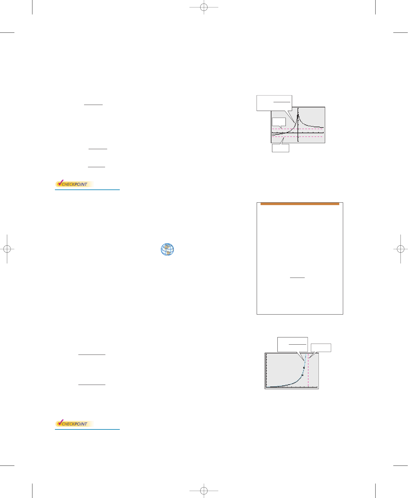
Horizontal and Vertical Asymptotes
In Example 1, the behavior of f near is denoted as follows.
decreases without bound as increases without bound as
approaches 0 from the left. approaches 0 from the right.
The line is a vertical asymptote of the graph of f, as shown in the figure
above. The graph of f has a horizontal asymptote—the line This means
the values of approach zero as increases or decreases without bound.
approaches 0 as approaches 0 as
decreases without bound. increases without bound.
Figure 3.43 shows the horizontal and vertical asymptotes of the graphs of
three rational functions.
x f
共
x
兲
x f
共
x
兲
f
共
x
兲
→ 0 as x →
f
共
x
兲
→ 0 as x →
x f
共
x
兲
1兾x
y 0.
x 0
xx
f
共
x
兲
f
共
x
兲
f
共
x
兲
→
as x → 0
f
共
x
兲
→
as x → 0
x 0
Section 3.5 Rational Functions and Asymptotes
299
Figure 3.43
Library of Parent Functions: Rational Function
A rational function is the quotient of two polynomials,
A rational function is not defined at values of for which Near
these values the graph of the rational function may increase or decrease
without bound. The simplest type of rational function is the reciprocal
function The basic characteristics of the reciprocal function
are summarized below. A review of rational functions can be found in the
Study Capsules.
Graph of
Domain:
Range:
No intercepts
Decreasing on and
Odd function
Origin symmetry
Vertical asymptote: -axis
Horizontal asymptote: -axis
x
y
共
0,
兲共
, 0
兲
共
, 0
兲
傼
共
0,
兲
共
, 0
兲
傼
共
0,
兲
123
1
2
3
y
x
f(x) =
1
x
Vertical
asymptote:
y-axis
Horizontal
asymptote:
x-axis
f
共
x
兲
1
x
f
共
x
兲
1兾x.
D
共
x
兲
0.x
f
共
x
兲
N
共
x
兲
D
共
x
兲
.
f
共
x
兲
Definition of Vertical and Horizontal Asymptotes
1. The line is a vertical asymptote of the graph of f if
or as either from the right or from the left.
2. The line is a horizontal asymptote of the graph of f if
as or
x →
.x →
f
共
x
兲
→ b
y b
x → a, f
共
x
兲
→
f
共
x
兲
→
x a
Horizontal
asymptote:
y = 2
Vertical
asymptote:
x = −1
y
x
f(x) =
2x + 1
x + 1
−1−2−3−41
1
2
3
4
f(x) =
4
x
2
+ 1
−1−2−3123
−1
1
2
3
4
5
Horizontal
asymptote:
y = 0
y
x
f(x) =
2
(x − 1)
2
y
x
−1−2234
−1
2
3
4
5
Vertical
asymptote:
x = 1
1
Horizontal
asymptote:
y = 0
Exploration
Use a table of values to deter-
mine whether the functions in
Figure 3.43 are continuous.
If the graph of a function has
an asymptote, can you conclude
that the function is not
continuous? Explain.
333371_0305.qxp 12/27/06 1:30 PM Page 299

300 Chapter 3 Polynomial and Rational Functions
−33
2
−2
f(x) =
2x
3x
2
+ 1
Horizontal
asymptote:
y = 0
Figure 3.44
−66
5
−3
f(x) =
2x
2
x
2
− 1
Horizontal
asymptote:
y = 2
Vertical
asymptote:
x = −1
Vertical
asymptote:
x = 1
Figure 3.45
Exploration
Use a graphing utility to com-
pare the graphs of
Start with a viewing window
in which and
then zoom out.
Write a convincing argument
that the shape of the graph of
a rational function eventually
behaves like the graph of
where
is the leading term of the
numerator and is the
leading term of the
denominator.
b
m
x
m
a
n
x
n
y a
n
x
n
兾b
m
x
m
,
10
≤
y
≤
10,
5
≤
x
≤
5
y
2
3x
3
2x
2
y
1
3x
3
5x
2
4x 5
2x
2
6x 7
y
1
and y
2
.
Vertical and Horizontal Asymptotes of a Rational Function
Let f be the rational function
where and have no common factors.
1. The graph of f has vertical asymptotes at the zeros of
2. The graph of f has at most one horizontal asymptote determined by
comparing the degrees of and
a. If the graph of f has the line (the -axis) as a
horizontal asymptote.
b. If the graph of f has the line as a horizontal
asymptote, where is the leading coefficient of the numerator and
is the leading coefficient of the denominator.
c. If the graph of f has no horizontal asymptote.
n
>
m,
b
m
a
n
y a
n
兾b
m
n m,
xy 0n
<
m,
D
共
x
兲
.N
共
x
兲
D
共
x
兲
.
D
共
x
兲
N
共
x
兲
f
共
x
兲
N
共
x
兲
D
共
x
兲
a
n
x
n
a
n1
x
n1
. . .
a
1
x a
0
b
m
x
m
b
m1
x
m1
. . .
b
1
x b
0
Example 2 Finding Horizontal and Vertical Asymptotes
Find all horizontal and vertical asymptotes of the graph of each rational function.
a. b.
Solution
a. For this rational function, the degree of the numerator is less than the degree
of the denominator, so the graph has the line as a horizontal asymptote.
To find any vertical asymptotes, set the denominator equal to zero and solve
the resulting equation for
Set denominator equal to zero.
Because this equation has no real solutions, you can conclude that the graph
has no vertical asymptote. The graph of the function is shown in Figure 3.44.
b. For this rational function, the degree of the numerator is equal to the degree of
the denominator. The leading coefficient of the numerator is 2 and the leading
coefficient of the denominator is 1, so the graph has the line as a
horizontal asymptote. To find any vertical asymptotes, set the denominator
equal to zero and solve the resulting equation for
Set denominator equal to zero.
Factor.
Set 1st factor equal to 0.
Set 2nd factor equal to 0.
This equation has two real solutions, and so the graph has the
lines and as vertical asymptotes, as shown in Figure 3.45.
Now try Exercise 13.
x 1x 1
x 1,x 1
x 1
x 1 0
x 1 x 1 0
共
x 1
兲共
x 1
兲
0
x
2
1 0
x.
y 2
3x
2
1 0
x.
y 0
f
共
x
兲
2x
2
x
2
1
f
共
x
兲
2x
3x
2
1
333371_0305.qxp 12/27/06 1:30 PM Page 300

Section 3.5 Rational Functions and Asymptotes 301
Example 4 Finding a Function’s Domain and Asymptotes
For the function f, find (a) the domain of f, (b) the vertical asymptote of f, and
(c) the horizontal asymptote of f.
Solution
a. Because the denominator is zero when solve this equation to
determine that the domain of f is all real numbers except
b. Because the denominator of f has a zero at and is not a zero of
the numerator, the graph of f has the vertical asymptote
c. Because the degrees of the numerator and denominator are the same, and the
leading coefficient of the numerator is 3 and the leading coefficient of the
denominator is , the horizontal asymptote of f is
Now try Exercise 19.
y
3
4
.4
x
3
冪
5
4
⬇ 1.08.
3
冪
5
4
x
3
冪
5
4
,
x
3
冪
5
4
.
4x
3
5 0,
f
共
x
兲
3x
3
7x
2
2
4x
3
5
Example 3 Finding Horizontal and Vertical Asymptotes
and Holes
Find all horizontal and vertical asymptotes and holes in the graph of
Solution
For this rational function the degree of the numerator is equal to the degree of the
denominator. The leading coefficients of the numerator and denominator are both
1, so the graph has the line as a horizontal asymptote. To find any vertical
asymptotes, first factor the numerator and denominator as follows.
By setting the denominator (of the simplified function) equal to zero, you
can determine that the graph has the line as a vertical asymptote, as shown
in Figure 3.46. To find any holes in the graph, note that the function is undefined
at and Because is not a vertical asymptote of the func-
tion, there is a hole in the graph at To find the y-coordinate of the hole,
substitute into the simplified form of the function.
So, the graph of the rational function has a hole at
Now try Exercise 17.
共
2,
3
5
兲
.
y
x 1
x 3
2 1
2 3
3
5
x 2
x 2.
x 2x 3.x 2
x 3
x 3
x 2 f
共
x
兲
x
2
x 2
x
2
x 6
共
x 1
兲共
x 2
兲
共
x 2
兲共
x 3
兲
x 1
x 3
,
y 1
f
共
x
兲
x
2
x 2
x
2
x 6
.
f(x) =
x
2
+ x − 2
x
2
− x − 6
Horizontal
asymptote:
y = 1
Vertical
asymptote:
x = 3
−5
−612
7
Figure 3.46
Values for which a rational function is undefined (the denominator is zero)
result in a vertical asymptote or a hole in the graph, as shown in Example 3.
Notice in Figure 3.46 that the
function appears to be defined at
Because the domain of
the function is all real numbers
except and you
know this is not true. Graphing
utilities are limited in their reso-
lution and therefore may not
show a break or hole in the graph.
Using the table feature of a
graphing utility, you can verify
that the function is not defined
at x 2.
x 3,x 2
x 2.
TECHNOLOGY TIP
333371_0305.qxp 12/27/06 1:30 PM Page 301
Applications
There are many examples of asymptotic behavior in real life. For instance,
Example 6 shows how a vertical asymptote can be used to analyze the cost of
removing pollutants from smokestack emissions.
302 Chapter 3 Polynomial and Rational Functions
Example 6 Cost-Benefit Model
A utility company burns coal to generate electricity. The cost (in dollars) of
removing % of the smokestack pollutants is given by
for Use a graphing utility to graph this function. You are a member
of a state legislature that is considering a law that would require utility companies
to remove 90% of the pollutants from their smokestack emissions. The current
law requires 85% removal. How much additional cost would the utility company
incur as a result of the new law?
Solution
The graph of this function is shown in Figure 3.48. Note that the graph has a
vertical asymptote at Because the current law requires 85% removal,
the current cost to the utility company is
Evaluate C
at
If the new law increases the percent removal to 90%, the cost will be
Evaluate C
a
t
So, the new law would require the utility company to spend an additional
Now try Exercise 39.
720,000 453,333 $266,667.
p 90.C
80,000
共
90
兲
100 90
$720,000.
p 85.C
80,000
共
85
兲
100 85
⬇ $453,333.
p 100.
0
≤
p
<
100.
C 80,000p兾
共
100 p
兲
p
C
Subtract 85% removal cost from
90% removal cost.
−20 20
6
−2
f(x) =
x + 10
⏐
x
⏐
+ 2
y = 1
y = −1
Figure 3.47
ⱍ
x
ⱍ
x for x
≥
0
ⱍ
x
ⱍ
x for x
<
0
0 120
6
C =
80,000p
100 − p
p = 100
1,200,000
0
85%
90%
Figure 3.48
Exploration
The table feature of a graphing
utility can be used to estimate
vertical and horizontal asymp-
totes of rational functions.
Use the table feature to find
any horizontal or vertical
asymptotes of
Write a statement explaining
how you found the asymptote(s)
using the table.
f
共
x
兲
2x
x 1
.
Example 5 A Graph with Two Horizontal Asymptotes
A function that is not rational can have two horizontal asymptotes—one to the left
and one to the right. For instance, the graph of
is shown in Figure 3.47. It has the line as a horizontal asymptote to the
left and the line as a horizontal asymptote to the right. You can confirm this
by rewriting the function as follows.
Now try Exercise 21.
f
共
x
兲
冦
x 10
x 2
x 10
x 2
, x
<
0
,
x
≥
0
y 1
y 1
f
共
x
兲
x 10
ⱍ
x
ⱍ
2
333371_0305.qxp 12/27/06 1:30 PM Page 302
Section 3.5 Rational Functions and Asymptotes 303
Example 7 Ultraviolet Radiation
For a person with sensitive skin, the amount of time (in hours) the person can
be exposed to the sun with minimal burning can be modeled by
where is the Sunsor Scale reading. The Sunsor Scale is based on the level of
intensity of UVB rays. (Source: Sunsor, Inc.)
a. Find the amounts of time a person with sensitive skin can be exposed to the
sun with minimal burning when and
b. If the model were valid for all what would be the horizontal asymptote
of this function, and what would it represent?
s
>
0,
s 100.s 10, s 25,
s
0
<
s
≤
120T
0.37s 23.8
s
,
T
Algebraic Solution
a. When
hours.
When
hours.
When
hour.
b. Because the degrees of the numerator and
denominator are the same for
the horizontal asymptote is given by the
ratio of the leading coefficients of the
numerator and denominator. So, the graph
has the line as a horizontal
asymptote. This line represents the short-
est possible exposure time with minimal
burning.
Now try Exercise 43.
T 0.37
T
0.37s 23.8
s
⬇ 0.61
T
0.37
共
100
兲
23.8
100
s 100,
⬇ 1.32
T
0.37
共
25
兲
23.8
25
s 25,
2.75
T
0.37
共
10
兲
23.8
10
s 10,
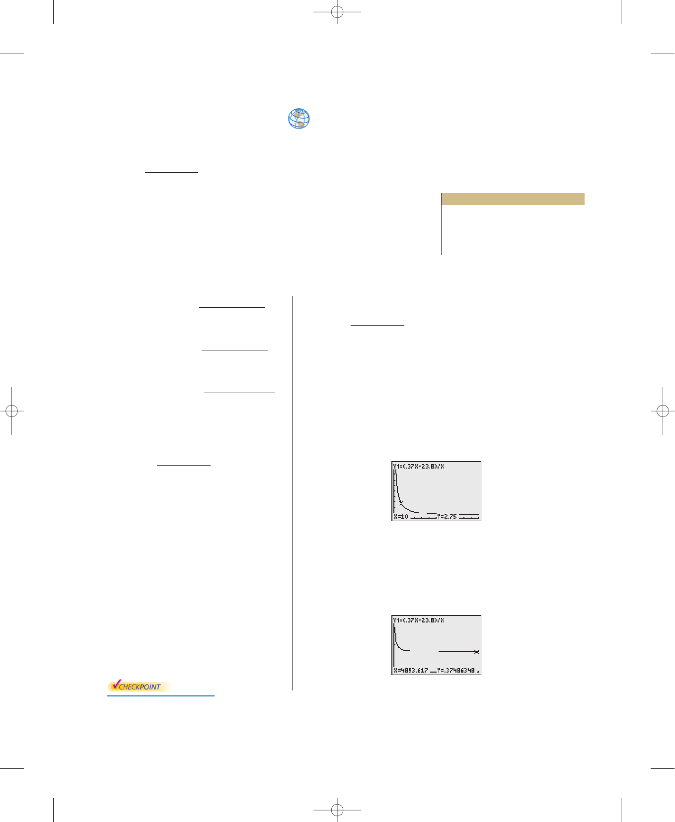
Graphical Solution
a. Use a graphing utility to graph the function
using a viewing window similar to that shown in Figure 3.49. Then
use the trace or value feature to approximate the values of when
and You should obtain the following
values.
When hours.
When hours.
When hour.
Figure 3.49
b. Continue to use the trace or value feature to approximate values of
for larger and larger values of (see Figure 3.50). From this, you
can estimate the horizontal asymptote to be This line
represents the shortest possible exposure time with minimal burning.
Figure 3.50
50000
0
1
y 0.37.
x f
共
x
兲
1200
0
1
0
y
1
⬇ 0.61x 100,
y
1
⬇ 1.32x 25,
y
1
2.75x 10,
x 100.x 10, x 25,
y
1
y
1
0.37x 23.8
x
For instructions on how to use the
value feature, see Appendix A;
for specific keystrokes, go to this
textbook’s Online Study Center.
TECHNOLOGY SUPPORT
333371_0305.qxp 12/27/06 1:30 PM Page 303

304 Chapter 3 Polynomial and Rational Functions
In Exercises 1–6, (a) find the domain of the function, (b)
complete each table, and (c) discuss the behavior of f near
any excluded x-values.
1. 2.
3. 4.
5. 6.
In Exercises 7–12, match the function with its graph. [The
graphs are labeled (a), (b), (c), (d), (e), and (f).]
(a) (b)
(c) (d)
(e) (f )
7. 8.
9. 10.
11. 12. f
共
x
兲
x 2
x 4
f
共
x
兲
x 2
x 4
f
共
x
兲
1 x
x
f
共
x
兲
4x 1
x
f
共
x
兲
1
x 3
f
共
x
兲
2
x 2
−10 2
−4
4
−66
−4
4
−48
−4
4
−78
−1
9
−210
−3
5
−84
−4
4
−66
−4
4
−66
−3
5
f
共
x
兲
4x
x
2
1
f
共
x
兲
3x
2
x
2
1
−78
−1
9
−12 12
−4
12
f
共
x
兲
3
ⱍ
x 1
ⱍ
f
共
x
兲
3x
ⱍ
x 1
ⱍ
−88
−6
12
−66
−4
4
f
共
x
兲
5x
x 1
f
共
x
兲
1
x 1
3.5 Exercises See www.CalcChat.com for worked-out solutions to odd-numbered exercises.
Vocabulary Check
Fill in the blanks.
1. Functions of the form where and are polynomials and is not the zero polynomial,
are called _______ .
2. If as from the left (or right), then is a _______ of the graph of f.
3. If as then is a _______ of the graph of f.y bx →
±
, f
共
x
兲
→ b
x ax → a f
共
x
兲
→
±
D
共
x
兲
D
共
x
兲
N
共
x
兲
f
共
x
兲
N
共
x
兲
兾D
共
x
兲
,
x
f
共
x
兲
0.5
0.9
0.99
0.999
x
f
共
x
兲
1.5
1.1
1.01
1.001
x
f
共
x
兲
5
10
100
1000
x
f
共
x
兲
5
10
100
1000
333371_0305.qxp 12/27/06 1:30 PM Page 304

Section 3.5 Rational Functions and Asymptotes 305
In Exercises 13– 18, (a) identify any horizontal and vertical
asymptotes and (b) identify any holes in the graph. Verify
your answers numerically by creating a table of values.
13. 14.
15. 16.
17. 18.
In Exercises 19–22, (a) find the domain of the function,
(b) decide if the function is continuous, and (c) identify any
horizontal and vertical asymptotes. Verify your answer to
part (a) both graphically by using a graphing utility and
numerically by creating a table of values.
19. 20.
21. 22.
Analytical and Numerical Explanation In Exercises 23–26,
(a) determine the domains of f and g, (b) simplify f and find
any vertical asymptotes of f, (c) identify any holes in the
graph of f, (d) complete the table, and (e) explain how the
two functions differ.
23.
24.
25.
26.
Exploration In Exercises 27–30, determine the value that
the function f approaches as the magnitude of x increases. Is
greater than or less than this function value when x is
positive and large in magnitude? What about when x is neg-
ative and large in magnitude?
27. 28.
29. 30.
In Exercises 31–38, find the zeros (if any) of the
rational function. Use a graphing utility to verify your
answer.
31. 32.
33. 34.
35.
36.
37.
38.
39. Environment The cost (in millions of dollars) of
removing of the industrial and municipal pollutants dis-
charged into a river is given by
(a) Find the cost of removing 10% of the pollutants.
(b) Find the cost of removing 40% of the pollutants.
(c) Find the cost of removing 75% of the pollutants.
(d) Use a graphing utility to graph the cost function. Be
sure to choose an appropriate viewing window. Explain
why you chose the values that you used in your view-
ing window.
(e) According to this model, would it be possible to
remove 100% of the pollutants? Explain.
0
≤
p
<
100.C
255p
100 p
,
p%
C
f
共
x
兲
2x
2
3x 2
x
2
x 2
f
共
x
兲
2x
2
5x 2
2x
2
7x 3
g
共
x
兲
x
2
5x 6
x
2
4
g
共
x
兲
x
2
2x 3
x
2
1
h
共
x
兲
5
3
x
2
1
f
共
x
兲
1
2
x 5
g
共
x
兲
x
3
8
x
2
4
g
共
x
兲
x
2
4
x 3
f
共
x
兲
2x 1
x
2
1
f
共
x
兲
2x 1
x 3
f
共
x
兲
2
1
x 3
f
共
x
兲
4
1
x
f
冇
x
冈
g
共
x
兲
x 2
x 1
f
共
x
兲
x
2
4
x
2
3x 2
,
g
共
x
兲
x 1
x 3
f
共
x
兲
x
2
1
x
2
2x 3
,
g
共
x
兲
x 3 f
共
x
兲
x
2
9
x 3
,
g
共
x
兲
x 4 f
共
x
兲
x
2
16
x 4
,
f
共
x
兲
x 1
ⱍ
x
ⱍ
1
f
共
x
兲
x 3
ⱍ
x
ⱍ
f
共
x
兲
3x
2
1
x
2
x 9
f
共
x
兲
3x
2
x 5
x
2
1
f
共
x
兲
3 14x 5x
2
3 7x 2x
2
f
共
x
兲
x
2
25
x
2
5x
f
共
x
兲
x
2
2x 1
2x
2
x 3
f
共
x
兲
x
共
2 x
兲
2x x
2
f
共
x
兲
3
共
x 2
兲
3
f
共
x
兲
1
x
2
x
1 2 3 4 5 6 7
f
共
x
兲
g
共
x
兲
x
0 1 2 3 4 5 6
f
共
x
兲
g
共
x
兲
x
2 1
0 1 2 3
4
f
共
x
兲
g
共
x
兲
x
3 2 1
0 1 2
3
f
共
x
兲
g
共
x
兲
333371_0305.qxp 12/27/06 1:30 PM Page 305

306 Chapter 3 Polynomial and Rational Functions
40. Environment In a pilot project, a rural township is given
recycling bins for separating and storing recyclable prod-
ucts. The cost
C
(in dollars) for supplying bins to of the
population is given by
(a) Find the cost of supplying bins to 15% of the popula-
tion.
(b) Find the cost of supplying bins to 50% of the popula-
tion.
(c) Find the cost of supplying bins to 90% of the popula-
tion.
(d) Use a graphing utility to graph the cost function. Be
sure to choose an appropriate viewing window. Explain
why you chose the values that you used in your view-
ing window.
(e) According to this model, would it be possible to supply
bins to 100% of the residents? Explain.
41. Data Analysis The endpoints of the interval over which
distinct vision is possible are called the near point and far
point of the eye (see figure). With increasing age these
points normally change. The table shows the approximate
near points (in inches) for various ages
(in years).
(a) Find a rational model for the data. Take the reciprocals
of the near points to generate the points Use
the regression feature of a graphing utility to find a lin-
ear model for the data. The resulting line has the form
Solve for
(b) Use the table feature of a graphing utility to create a
table showing the predicted near point based on the
model for each of the ages in the original table.
(c) Do you think the model can be used to predict the near
point for a person who is 70 years old? Explain.
42. Data Analysis Consider a physics laboratory experiment
designed to determine an unknown mass. A flexible metal
meter stick is clamped to a table with 50 centimeters over-
hanging the edge (see figure). Known masses ranging
from 200 grams to 2000 grams are attached to the end of
the meter stick. For each mass, the meter stick is displaced
vertically and then allowed to oscillate. The average time
(in seconds) of one oscillation for each mass is recorded in
the table.
A model for the data is given by
(a) Use the table feature of a graphing utility to create a
table showing the estimated time based on the model
for each of the masses shown in the table. What can you
conclude?
(b) Use the model to approximate the mass of an object
when the average time for one oscillation is
1.056 seconds.
t
38M 16,965
10
共
M 5000
兲
.
M
50 cm
t
M
y.1兾y ax b.
共
x, 1兾y
兲
.
Object
blurry
Object
blurry
Object
clear
Near
point
Far
point
xy
0
≤
p
<
100.C
25,000p
100 p
,
p%
Age, x Near point, y
16 3.0
32 4.7
44 9.8
50 19.7
60 39.4
Mass, M Time, t
200 0.450
400 0.597
600 0.712
800 0.831
1000 0.906
1200 1.003
1400 1.088
1600 1.126
1800 1.218
2000 1.338
333371_0305.qxp 12/27/06 1:30 PM Page 306

Section 3.5 Rational Functions and Asymptotes 307
43. Wildlife The game commission introduces 100 deer into
newly acquired state game lands. The population of the
herd is given by
where is the time in years.
(a) Use a graphing utility to graph the model.
(b) Find the populations when and
(c) What is the limiting size of the herd as time increases?
Explain.
44. Defense The table shows the national defense outlays
(in billions of dollars) from 1997 to 2005. The data can be
modeled by
where t is the year, with corresponding to 1997.
(Source: U.S. Office of Management and Budget)
(a) Use a graphing utility to plot the data and graph the
model in the same viewing window. How well does the
model represent the data?
(b) Use the model to predict the national defense outlays
for the years 2010, 2015, and 2020. Are the predictions
reasonable?
(c) Determine the horizontal asymptote of the graph of the
model. What does it represent in the context of the
situation?
Synthesis
True or False? In Exercises 45 and 46, determine whether
the statement is true or false. Justify your answer.
45. A rational function can have infinitely many vertical
asymptotes.
46. A rational function must have at least one vertical
asymptote.
Library of Parent Functions In Exercises 47 and 48,
identify the rational function represented by the graph.
47. 48.
(a) (a)
(b) (b)
(c) (c)
(d) (d)
Think About It In Exercises 49– 52, write a rational func-
tion f that has the specified characteristics. (There are many
correct answers.)
49. Vertical asymptote:
Horizontal asymptote:
Zero:
50. Vertical asymptote:
Horizontal asymptote:
Zero:
51. Vertical asymptotes:
Horizontal asymptote:
Zeros:
52. Vertical asymptotes:
Horizontal asymptote:
Zeros:
Skills Review
In Exercises 53–56, write the general form of the equation
of the line that passes through the points.
53. 54.
55. 56.
In Exercises 57–60, divide using long division.
57.
58.
59.
60.
共
4x
5
3x
3
10
兲
共
2x 3
兲
共
2x
4
x
2
11
兲
共
x
2
5
兲
共
x
2
10x 15
兲
共
x 3
兲
共
x
2
5x 6
兲
共
x 4
兲
共
0, 0
兲
,
共
9, 4
兲共
2, 7
兲
,
共
3, 10
兲
共
6, 1
兲
,
共
4, 5
兲共
3, 2
兲
,
共
0, 1
兲
x 2, x 3
y 2
x 1, x 2
x 3, x 3
y 2
x
2, x 1
x 2
y 0
x 1
x 1
y 0
x 2
f
共
x
兲
x
x
2
1
f
共
x
兲
x 9
x
2
4
f
共
x
兲
x
x
2
1
f
共
x
兲
x 4
x
2
9
f
共
x
兲
x
2
1
x
2
1
f
共
x
兲
x
2
4
x
2
9
f
共
x
兲
x
2
1
x
2
1
f
共
x
兲
x
2
9
x
2
4
x
y
−1123
3
−4246
−4
−6
2
4
6
x
y
t 7
7
≤
t
≤
15D
1.493t
2
39.06t 273.5
0.0051t
2
0.1398t 1
,
D
t 25.t 5, t 10,
t
t
≥
0N
20
共
5 3t
兲
1 0.04t
,
N
Year
Defense outlays
(in billions of dollars)
1997 270.5
1998 268.5
1999 274.9
2000 294.5
2001 305.5
2002 348.6
2003 404.9
2004 455.9
2005 465.9
333371_0305.qxp 12/27/06 1:30 PM Page 307
