
ISSN: 1962-5361
Disclaimer: This Philadelphia Fed working paper represents preliminary research that is being circulated for discussion purposes. The views
expressed in these papers are solely those of the authors and do not necessarily reflect the views of the Federal Reserve Bank of
Philadelphia or the Federal Reserve System. Any errors or omissions are the responsibility of the authors. Philadelphia Fed working papers
are free to download at: https://philadelphiafed.org/research-and-data/publications/working-papers.
Working Papers
Using High-Frequency Evaluations
to Estimate Discrimination: Evidence
from Mortgage Loan Officers
Marco Giacoletti
University of Southern California
Rawley Z. Heimer
Boston College
Edison G. Yu
Federal Reserve Bank of Philadelphia Research Department
WP 21-04
Revised April 2021
February 2021
https://doi.org/10.21799/frbp.wp.2021.04

Using High-Frequency Evaluations to Estimate Discrimination:
Evidence from Mortgage Loan Officers
∗
Marco Giacoletti
†
USC
Rawley Z. Heimer
‡
Boston College
Edison G. Yu
§
FRB-Philadelphia
Current Draft: March 1, 2021
First Draft: August 24, 2020
Abstract
We develop empirical tests for discrimination that use high-frequency evaluations to address
the problem of unobserved heterogeneity in a conventional benchmarking test. Our approach
to identifying discrimination requires two conditions: (1) the subject pool is time-invariant in
a short time horizon and (2) there is high-frequency variation in the extent to which evaluators
can rely on their subjective assessments. We bring our approach to the residential mortgage
market, using data on the near-universe of U.S. mortgage applications from 1994 to 2018.
Monthly volume quotas reduce how much subjectivity loan officers apply to loans they process
at the end of the month. As a result, the volume of new originations increases by 150% at the
end of the month, while application volume and applicants’ quality are constant within the
month. Owing to within-month variation in loan officers’ subjectivity, we estimate that Black
mortgage applicants have 3.5% to 5% lower approval rates, which explains at least half of the
observed approval gap for Blacks. When we use this approach to evaluate policies, we find
that market concentration and FinTech lending have had no effect on lending discrimination,
but that shadow banking has reduced discrimination presumably by having a larger presence
in under-served communities.
Keywords: Performance Incentives, Loan Officers, Mortgages, FinTech Lending, Lend-
ing Discrimination
∗
Previously titled “To the Back of the (Lending) Bus: How Loan Officers’ Performance Incentives Reveal Lend-
ing Discrimination.” We thank Michael Fitzpatrick for excellent research assistance. We thank Pat Akey, Mitchell
Berlin, Greg Buchak, Yulyia Demyanak, Ran Duchin, Andreas Fuster, Antonio Gargano, Hajime Hadeishi, Chris
Parsons, Micah Spector, Phil Strahan, and seminar participants at Baruch, ASU Finance Winter Conference, Boston
College, Federal Reserve Bank of Philadelphia, the Joint Finance Seminar, University of Oregon, and University
of Southern California for helpful feedback. This paper does not reflect the views of the Federal Reserve Bank of
Philadelphia or of the Federal Reserve System. Any remaining errors or omissions are the authors’ responsibility.
†
University of Southern California, Marshall School of Business. Phone: +1 (650) 475-6410, Email: mgia-
‡
§
1 Introduction
Racial and gender disparities have been documented in a range of fields, such as labor markets,
the legal system, and credit markets. Yet whether these disparities are the result of discrimination
by economic decision-makers—defined as an evaluator treating otherwise identical subjects from
minority groups worse than subjects from the majority group—remains in dispute. There has been
a growing trend toward using experiments and correspondence studies to test for discrimination
(Bertrand and Duflo, 2017). Nonetheless, tests for discrimination that use observational data have
several advantageous features. Such tests are accessible to a wide range of researchers, they are
easy to replicate and scale, they can be used to estimate aggregate costs of discrimination in a given
market, and policymakers can easily implement them.
However, tests for discrimination based on observational data face a number of economet-
ric challenges that limit their appeal. The most straightforward test for discrimination is an audit
or “benchmarking” test. Benchmarking tests claim to find discrimination when minority groups
receive unfavorable evaluations relative to the majority group. But, benchmarking tests are vul-
nerable to criticisms of omitted variable bias—differences in group characteristics, which the re-
searcher does not observe, can cause differences in evaluations across groups.
Alternatively, Becker (1957) proposed an “outcome test.” Instead of comparing differences
in how groups are evaluated, outcome tests compare the ex-post success of these evaluations.
The marginal minority will have better ex-post outcomes than the marginal majority subject be-
cause minority groups face higher thresholds for inclusion when they are subject to discrimination.
Though intuitively appealing, outcome tests are notoriously difficult to implement, most notably
because of the “infra-marginality” problem—the average difference in ex-post outcomes can be
a poor approximation of the difference in marginal outcomes (Ayres, 2002). Recent research has
made significant progress to improve econometric methods (e.g., Arnold et al., 2018), but address-
ing the infra-marginality problem requires additional modelling and distributional assumptions
(Simoiu et al., 2017). Furthermore, ex-post outcomes can be the result of self-fulfilling prophecies
1

(e.g., female students underperform in math because gender stereotypes reduce investment in fe-
males’ math education; Bordalo et al., 2016) and ex-post outcomes are often not easily measured
(e.g., worker productivity can be difficult to measure and proxies for productivity, such as wages,
can also be affected by discrimination).
We propose an alternative way to test for discrimination. The approach is motivated by the
observation that evaluators’ subjectivity can often vary substantially within short time intervals.
For example, employers that have immediate staffing needs can ill afford to turn away job appli-
cants. TSA agents might reduce their screening of travelers when they are at the end of their shifts
or there are long queues. Police officers that have monthly quotas would issue tickets to all drivers
that exceed the speed limit on the last day of the month. Our approach starts with a benchmarking
test, but addresses the problem of omitted variables by exploiting such high-frequency evaluations.
The approach requires two simple assumptions: time-varying discrimination and time-invariant
unobserved characteristics both in a short time interval (e.g., a month). The identification ratio-
nale is straightforward. If the evaluations of a group vary within a short time interval, then these
differences cannot be driven by unobserved subject characteristics, because the unobserved char-
acteristics are time-invariant.
We apply our approach to high-frequency data on mortgage applications, to test for discrim-
ination in the U.S. residential mortgage market.
1
We obtain the time-stamped version of the Home
Mortgage Disclosure Act (HMDA) data, covering the near-universe of mortgage applications from
1994 to 2018 with 500 million loan applications across more than 28,000 lenders. Crucial to our
empirical approach, we observe the exact application and decision date of each application.
Figure 1 demonstrates our key source of high-frequency variation in the mortgage market
and the foundation of our empirical approach. The figure shows the volume of new originations
and new applications relative to the first day of a given month. The total volume of new mortgage
originations increases by more than 150% on the last day relative to the first day of a given month.
1
The literature can be traced back at least as far as the public release of HMDA data and the work of Munnell
et al. (1996). Ladd (1998) summarizes much of the older literature and frames longstanding debates. Other founda-
tional papers include Berkovec et al. (1994); Tootell (1996); Berkovec et al. (1998). Recent work has begun to study
differences in mortgage rates and fees (e.g., Bhutta and Hizmo, 2020).
2

0
50
100
150
200
percent
-7 -6 -5 -4 -3 -2 -1 0 1 2 3 4 5 6 7
days around last day of month
origination application
Number of loans originated vs applied (relative to first day of month)
Figure 1: The figure shows average percentage abnormal daily loan origination volume, and loan application vol-
ume (measured as number of originations and applications) in the U.S., for the last eight days of the month, and the
first seven days of the following month. The figure reports the average across all months over the sample period from
January 1994 to December 2018 from the HMDA data. Abnormal volume is computed with respect to loan origina-
tions and applications on the first day of the following month.
At the same time, the number of submitted mortgage applications stays constant over the course of
the month. These patterns reveal a crucial feature of the mortgage application process: loans are
processed by individual loan officers who have monthly performance targets that determine their
compensation.
2
Moreover, this within-month pattern in loan approvals unveils the component of
loan officers’ decision-making that is orthogonal to observable and unobservable factors affecting
loan originations (e.g., credit market conditions, applicant characteristics, and firm-level charac-
teristics). Drawing from Becker (1957), a profit-maximizing agent can give disparate treatment
to minority populations until market competition makes discrimination economically untenable.
2
Though we do not directly measure the compensation of any individual loan officer, for the most part, com-
missions are set based on the number of loans and the loan amount originated. And the compensation scheme
is common across employers. For example, see the following link for an article on the website of the Mort-
gage Bankers Association that discusses the industry standards for loan officers’ compensation in the U.S.
(https://www.mba.org/publications/insights/archive/mba-insights-archive/2019/is-it-time-to-rethink-compensation-
x253848). Tzioumis and Gee (2013) also note that loan officers face disciplinary actions if they fail to meet their
quotas several months in a row. Given this non-linear incentive scheme, Tzioumis and Gee (2013) and Cao et al.
(2020) document end-of-month bunching in a large U.S. commercial bank and in two Chinese banks, respectively.
3

Loan officers have an economic incentive to meet end-of-month performance incentives. As such,
loan officers’ subjective favoritism toward applicants has to attenuate at the end of the month
relative to the beginning of the month. Therefore, the within-month pattern, combined with a con-
ventional benchmark test, allows us to estimate the extent to which loan approval decisions can be
attributed to loan officers’ subjectivity towards applicants.
-.25
-.2
-.15
-.1
-7 -6 -5 -4 -3 -2 -1 0 1 2 3 4 5 6 7
days around last day of month
Average approval rate gap (Black minus white applications)
Figure 2: The figure reports the difference between the fraction of approved loans, out of all approved and denied
loans in the U.S., for Blacks minus the one for whites, on each of the last eight days of the month and the first seven
days of the following month.
Exploiting this within-month variation, our tests for discrimination estimate the difference in
approval rates between Black and white applicants at the start of the month relative to the end of
the month. Our key finding is summarized in Figure 2, which shows the difference in application
approval rates between Black and white applicants over the course of any given month. In the first
seven days of the month, Black applicants have 20 percentage point lower approval rates than white
applicants. The approval gap gets smaller over the course of the month. The approval gap between
Blacks and whites is just 10 percentage points on the last day of the month. The regression tests that
correspond to the graphical evidence in Figure 2 are saturated with a rich set of fixed effects that
control for time-varying economic conditions at precise geographic levels, namely county-month.
4

The regressions also include lender-month fixed effects that control for factors, such as regulations,
that would affect lending at the institution level. Confirming the graphical evidence, the difference
in the Black-white approval gap between the start and the end of the month is 3 to 5 percentage
points. This constitutes a lower bound on the share of the Black-white approval gap that is due
to loan officers’ subjectivity, relative to the approval gap that can be attributed to unobservable
group-differences. We estimate, in our most stringent regressions, that loan officers’ subjective
decision-making explains at least half of the overall difference in approval rates between Black
and white applicants even after controlling for observable characteristics. In terms of aggregate
magnitudes, if the approval rate gap for every day of the month was as small as the last day of the
month, about 1.4 million more Black applications would have been approved rather than denied
between 1994 and 2018, which corresponds to a total loan size of about $213 billion in 2018
dollars.
Our approach to estimating discrimination hinges on a set of simple assumptions that we de-
rive and that are easily supportable, either in the data or via narrative, or both. The first assumption
is that the loan officer has time-varying costs of being subjective. In our setting, loan officers have
nonlinear contract incentives.
3
Loan officers that fail to meet their volume quotas will have re-
duced compensation and risk getting fired. The second assumption is that the characteristics of the
subject pool are time invariant. Indeed, we find that application volume, the relative share of Black
applications, and loan application quality (for both Black and white applications) are all constant
over the course of the month. The remaining threat to identification is that there are differential
trends by race in the quality of applications that get processed over the course of the month. As
evidence against this explanation, we find that high-quality and low-quality Black mortgages have
similar amounts of bunching toward the end of the month.
3
Importantly, with volume quotas, the optimal strategy would be to approve all loan applications. However, in
practice, there are several constraints on this strategy. Lenders set origination standards that an application has to
exceed and loan officers may have a fixed quantity of mortgage credit that they can distribute within a month. Loan
officers can use their discretion and work to sidestep the origination standards by either using risk-based pricing or
appealing to other “soft” criteria, such as noting that the applicant is a customer of the bank.
5
In contrast to other methodologies, our approach does not require ex-post outcomes to test
for discrimination. Nevertheless, we show that a conventional outcome test is potentially mislead-
ing about the levels of discrimination in mortgage lending. We find that Black mortgages have
significantly higher rates of default, which could be interpreted as evidence of reverse discrimina-
tion that favors minorities. Instead, this result is almost certainly caused by the infra-marginality
problem – the fact that Black and white mortgage applicants have different risk distributions. We
compare the subsequent default rates of applications approved at the start of the month to those
approved at the end of the month. The within-month differential significantly shrinks the raw dif-
ference between Black and white default rates. As such, these findings suggest that our approach
potentially counteracts the shortcomings of a conventional outcome test.
Furthermore, our approach offers guidance, relative to both benchmarking and outcome tests,
as to whether observed discrimination is caused by taste-based versus statistical discrimination. We
develop an additional set of assumptions to distinguish between the two theories. Put simply, the
case for statistical discrimination requires asymmetric information between evaluators and sub-
jects. Because of the high-frequency nature of our data, statistical discrimination would require
the loan officers’ information set about applicants to change from the start to the end of the month.
This explanation is unlikely because we show that the applicant pool is time invariant. Related,
we consider the role of inaccurate beliefs (i.e., stereotypes Bordalo et al., 2016) and a similar logic
precludes this explanation.
Finally, our approach is advantageous because it can easily be applied to evaluate the effect
of market policies and market innovations on the quantity of discrimination. We consider three im-
portant features of modern mortgage lending: market concentration in banking, FinTech lending,
and shadow banking. We find that the amount of discrimination due to loan officers’ subjectivity
is unaffected by both market concentration and FinTech lending. This result is largely consistent
with the fact that our regressions include lender-by-month fixed effects and that the component
of loan officer subjectivity our approach uncovers occurs within-lender. Moreover, despite these
changes to the banking sector, loan officer compensation incentives have largely remained con-
6

stant throughout our sample, and even mortgage lending at FinTech lenders involves significant
discretion from human loan officers. On the other hand, we find that shadow banks have lower
levels of subjective discrimination against Black applicants. This is likely the result of shadow
banks—owing to their lower regulatory requirements—having a larger presence in under-served
communities.
Related Literature
Our paper is related to advances in the literature on identifying discrimination by economic decision-
makers. Our approach bears closest resemblance to empirical papers that use changes to evaluation
settings to identify discrimination against minority groups. For example, Goldin and Rouse (2000)
shows that blind auditions reduce employment discrimination against female orchestra musicians.
Police officers are less likely at night than during the day to pull over Black motorists because
the driver’s race is difficult to identify (Pierson et al., 2020). These empirical papers identify
discrimination by comparing situations in which evaluators know the subject’s gender and race to
situations in which they do not. Our approach is different because there is no change in the loan of-
ficer’s knowledge of applicants’ race. We show that discrimination can be identified under a set of
simple assumptions about the applicant pool and loan officers’ reliance on subjective assessments.
More specifically, our paper joins a large and important literature on discriminatory lending
practices in consumer credit markets. Our empirical approach is grounded in evidence that loan
officers have significant discretion in loan processing decisions (see e.g., Engelberg et al., 2012;
Chen et al., 2016; Demiroglu et al., 2019). Most similar to our analysis, Cort
´
es et al. (2016) also use
confidential HMDA data to disentangle application dates from processing dates to show that loan
officers are more likely to approve mortgages on sunny days. Guided by this finding, we bring the
confidential HMDA data to the question of lending discrimination. Several papers find compelling
evidence that individual loan officers discriminate against other races and women.
4
We advance
4
In no particular order, Fisman et al. (2017, 2020) use data from Indian banks to show that loan officers are more
favorable to culturally proximate applicants. Beck et al. (2018) use evidence from an Albanian bank and Montoya
et al. (2019) use a field experiment at a Chilean bank to uncover evidence of gender discrimination in consumer lend-
ing. Ambrose et al. (2020) find that minorities pay higher fees when they have a white mortgage broker.
7
this literature in a few ways. With a few exceptions (e.g., Bohren et al., 2019; Dobbie et al., 2020),
most papers are unable to distinguish between taste-based and statistical discrimination. Our ap-
proach can offer guidance about which type of discrimination is most likely. Also, these papers use
evidence from confidential internal data from one or two lending institutions. In contrast, our paper
uses the universe of U.S. mortgage applications over a 25-year period to connect racial disparities
in lending to the incentives of individual loan officers. This allows us to address crucial questions
about external validity, investigate the effects of the market structure, and quantify the scope of
racial bias in mortgage markets.
Second, our paper contributes to a growing literature on how market structure and technology
affect consumer lending. First, recent papers find support for classic theories arguing that compe-
tition reduces discrimination in consumer lending (Buchak and Jørring, 2017; Butler et al., 2019).
Such papers suggest that racial discrimination declines because of changes to the composition of
lending institutions. We find that discrimination by individual decision-makers can persist within
organizations even when there are differences in institution-level competition across markets. Sec-
ond, there is significant debate over how the growth of FinTech lending affects the allocation of
credit, with a particular interest in the effects on disadvantaged borrowers. In theory, FinTech can
reduce intermediation costs which can pass through to consumers (e.g., Tang, 2019) or improve
screening (Berg et al., 2020a). However, the literature finds that FinTech algorithms have either no
effect or negative effects on the supply of credit to disadvantaged consumers (see e.g., Fuster et al.,
2017; Bartlett et al., 2019). Our contribution is to show that biases in human decision-making can
survive advances in loan processing technology (similar to findings on the introduction of machine
learning to judicial outcomes, as shown by Kleinberg et al., 2018).
Finally, we make a unique contribution to the literature on performance-based compensation,
with a particular focus on financial intermediation. The effects of performance-based compensa-
tion have been studied in a range of settings, such as manufacturing (Oyer, 1998), software sales
(Larkin, 2014), government contracts (Liebman and Mahoney, 2017), healthcare (Li et al., 2014;
Gravelle et al., 2010), firm managers (Bandiera et al., 2007) and accounting (Murphy, 2000). The
8
literature has also studied how performance incentives within banks affect loan officers’ effort
and performance (Agarwal and Ben-David, 2012; Cole et al., 2015), and information production
(Hertzberg et al., 2010; Qian et al., 2015; Berg et al., 2020b). To the best of our knowledge, our
paper is the first to study variation in performance incentives combined with racial biases in human
decision-making.
2 Identifying Discrimination
This section presents a formal discussion of our empirical setup. We compare our approach to
existing frameworks for identifying discrimination. Differences in unobserved characteristics of
different subject groups pose a challenge for conventional tests for discrimination. Our approach
is to filter out these unobserved differences across subject groups by using high frequency data.
Our approach extends conventional tests for discrimination, called either audit or bench-
marking. These tests compare the conditional likelihood that a minority subject group receives
disparate treatment relative to the majority group, after controlling for other observable character-
istics from the point of view of the researcher. Consider the case of a Black mortgage applicant.
The researcher claims to have uncovered discrimination when she rejects the null of no difference
in the conditional likelihood of approval between Blacks and whites, and instead finds that the
likelihood is significantly smaller for Blacks. Specifically, the researcher claims discrimination
when she finds that:
P (a|W, X) > P (a|B, X) (1)
where P (a|R, X) is the probability of loan application approval, conditional on race R ∈ {W, B}
(white or Black) and a vector of observable characteristics X to the researcher. However, this
approach is exposed to the criticism that the difference in approval rates between white and Black
applicants might be driven by unobserved characteristics that are relevant for the assessment of
applicants’ credit risk used by the loan officers, but are not included in the vector of controls X
9
used by the researcher. To see that, assume for simplicity that there is a binary unobserved variable
Z ∈ {Z
L
, Z
H
}, such that the following assumptions are satisfied:
Assumptions Set (A)
No discrimination: P (a|W, X, Z
k
) = P (a|B, X, Z
k
)
for k ∈ {H, L}
Higher quality predicts higher approval probability: P (a|R, X, Z
H
) > P (a|R, X, Z
L
)
On average white applicants have better unobservables: P (Z
H
|W, X) > P (Z
L
|B, X)
The inequality in approval rates formalized by equation (1) holds under the set assumptions above
when omitting the variable Z, even though decision-makers do not discriminate when all of the
characteristics are accounted for (see Appendix A.I). The differences in approval rates for dif-
ferent races simply capture the differences in the unobserved characteristics. In the mortgage-
lending setting, Black and white applicants have substantially different observable characteristics
(see Table 1). Such differences raise concern that there might be also substantial differences in
unobservables.
In this paper, we show that we can refine existing approaches to address the identification
problems due to the systematic differences in unobservables across subject groups. Rather than
only testing for the differences in the likelihood of approval between white and Black applicants,
we use high-frequency data to test whether those differences vary over a short period of time.
Because discrimination is determined by the subjective judgment of the evaluators, under the null
of no discrimination, and if applicant characteristics remain constant over time, there shall be no
change in the approval rates over time. On the other hand, discrimination would predict a change
in the relative approval rates over time.
To formalize this idea, let there be two time periods, T ∈ {Start, End}. Assume that
evaluators have more scope to be subjective in period Start relative to period End. Then, in the
10
presence of time-varying discrimination we expect to find:
P (a|W, X, End) − P (a|B, X, End) < P (a|W, X, Start) − P (a|B, X, Start) (2)
where P (a|., X, .) is the probability of approval, conditional on race (white or Black), a vector of
observable characteristics X, and in a specific period (Start or End). Note that the presence of
unobservable quality characteristics systematically correlated with race cannot alone explain the
effects in equation (2). Consider the following set of assumptions that characterize a situation in
which there is no discrimination:
Assumptions Set (B)
No discrimination: P (a|W, X, Z
k
, T ) = P (a|B, X, Z
k
, T )
for k ∈ {H, L}
Higher quality predicts higher approval probability: P (a|X, Z
H
, T ) > P (a|X, Z
L
, T )
On average white applicants have better unobservables: P (Z
H
|W, T ) > P (Z
H
|B, T )
No time pattern in applications quality: P (Z
H
|R, X, Start) = P (Z
H
|R, X, End)
The first three assumptions are the same as in Assumptions Set (A), while the last assumption
states that the unobserved characteristics of the applicants, for both whites and Blacks, are on
average constant over time. Jointly, these assumptions imply (see Appendix A.I):
P (a|W, X, End) − P (a|B, X, End) = P (a|W, X, Start) − P (a|B, X, Start).
Thus, the condition in equation (2) indeed amounts to a rejection of the null of no discrimination.
2.1 Distinguishing Taste-Based from Statistical Discrimination
This section explores the extent to which our approach can distinguish between the two broad
categories of discrimination. Under “taste-based” discrimination, minorities are subject to dis-
parate treatment because evaluators have animus toward them. Under “statistical” discrimination,
11
evaluators are uncertain about the abilities of any given subject. Evaluators form their beliefs after
observing the subject’s race. Minorities are subject to disparate treatment when evaluators have de-
veloped beliefs that minority subjects have worse abilities. Evaluators do not need to have accurate
beliefs about minorities to apply disparate treatment (see e.g., Bohren et al., 2020).
We consider evaluators j who, over a short time-period, for example a month or a week,
evaluate subjects i. Each evaluator j has perceived net benefits from making decisions that favor
subject i equal to U
j
(X
i
, Z
i
, R
i
, t), where X
i
and Z
i
are vectors of observable and unobservable
(from the perspective of the researcher) characteristics, R
i
is the subjects’ race (e.g., R
i
= W
for a white applicant and R
i
= B for a Black applicant), and t is the point in time in which the
evaluation is conducted.
The evaluator’s net benefits can be decomposed into two components:
U
j
(X
i
, Z
i
, R
i
, t) = b
j
(X
i
, Z
i
, R
i
, t) + E
j
[u
i
|X
i
, Z
i
, R
i
, t], (3)
where b
j
(X
i
, Z
i
, r
i
, t) is the subjective net benefits of evaluator j conditional on all characteristics,
and E
j
[u
i
|V
i
, Z
i
, R
i
, t] is the statistical component. The statistical component can be written as
E
j
[u
i
|X
i
, Z
i
, R
i
, t] = E[u
i
|X
i
, Z
i
, R
i
, t] + τ
j
(R
i
, t), (4)
where τ
j
(.) is the bias of decision maker j when forming expectations conditional only on the
information about the race of an applicant.
We can then use our stylized framework to characterize different types of discrimination, for
example against Black subjects with respect to white subjects:
- Taste-based discrimination: b
j
(X
i
, Z
i
, W, t) > b
j
(X
i
, Z
i
, B, t)
- Statistical discrimination: τ
j
(W, t) > τ
j
(B, t)
12
The decision maker will take a decision favorable to subject i as long as the net benefit is
positive:
b
j
(X
i
, Z
i
, R
i
, t) + E
j
[u
i
|X
i
, Z
i
, R
i
, t] + v
i,j,t
> 0,
where v
i,j,t
is a random preference shock, i.i.d. across subjects and evaluators, and independent of
information on subject characteristics and evaluators’ beliefs. We can then introduce the variable
y
i,j,t
, which is equal to one if subject i receives a favorable decision from evaluator j at time t, and
has likelihood function:
L(y
i,j,t
) = P r(y
i,j,t
= 1)
I(y
i,j,t
=1)
[1 − P r(y
i,j,t
= 1)]
1−I(y
i,j,t
=1)
P r(y
i,j,t
= 1) = E[y
i,j,t
|X
i
, Z
i
, R
i
, j, t] = F (X
i
, Z
i
, R
i
, j, t).
If we assume the function F (X
i
, Z
i
, R
i
, j, t) can be approximated with a liner specification,
then we can write:
y
i,j,t
= β
1
r
i
+ β
2
(r
i
× t) + ηX
i
+ φZ
i
+ a
t
+
i,j,t
(5)
where r
i
= 1 if R
i
= B. Equation (5) can be estimated in the data. Within this specific framework,
we can state the predictions of our general discussion in the previous section along the following
lines:
1. The two types of discrimination listed above (driven by taste or statistical) would cause
estimates of β
1
< 0. However, as the previous section outlines, β
1
will be a biased estimate
unless the researcher fully controls for observable (X
i
) and unobservable (Z
i
) characteristics,
or r
i
is uncorrelated with any omitted characteristics.
2. Estimates of β
2
will be different from zero if the magnitude of discrimination changes over
time, regardless of the type of discrimination. If subject pool characteristics (X
i
and Z
i
)
are not correlated with the evaluation time t, estimates of β
2
will be unbiased even if the
researcher does not perfectly control for time-invariant characteristics.
13
How can this approach distinguish between different theories of discrimination? In principle,
any type of discrimination can be subject to high-frequency fluctuations, and thus produce non-
zero estimates of β
2
. However, if the unobserved variation across subject pools and the evaluator’s
statistical inference problem are time-invariant, our approach allows the researcher to attribute
discrimination to the source of time-variation in the evaluator’s decision-making.
Consider the case of statistical discrimination. Statistical discrimination is caused by the
evaluators’ statistical inference problem. Therefore, the researcher can reasonably assume the
findings are caused by statistical discrimination if she can provide evidence of time-variation in the
evaluators’ information set. Now consider taste-based discrimination. The evaluator’s subjective
preferences against minorities causes disparate treatment. The researcher can assume taste-based
discrimination if she has evidence that evaluators’ subjectivity is time-varying.
In the following empirical analysis, we focus on residential mortgage lending in the U.S.
Our source of time-variation in evaluations is the fact that loan officers have monthly volume quo-
tas. These monthly volume quotas generate within-month variation in loan officers’ subjectivity.
The volume quotas pressure loan officers to increase their approval rates at the end of the month,
whereas at the start of the month, loan officers have scope to apply their subjective preferences. At
the same time, loan officers observe the same information about applications that they process at
the start of the month relative to the end of the month. As such, any finding of discrimination due to
within-month differences in evaluations can be attributed to loan officers’ subjective preferences.
3 Data
The empirical results in this paper are based on the confidential version of the HMDA data available
to researchers in the Federal Reserve System. The dataset contains the largest sample of mortgage
applications available in the U.S. The public version of the data includes information on applicant
characteristics – race, gender, reported income, and location of the property – and identifiers for
the lenders that received the applications. The data cover the entire geography of the U.S. over
the period from January 1994 through December 2018. Moreover, the data provide information on
14

mortgage contract characteristics, such as whether the application is for a new home purchase or
refinancing, the loan amount, the lien, and whether the property is owner-occupied. The primary
distinguishing feature of the confidential version of the HMDA data is that it contains the exact
date on which each application was submitted by a potential borrower and the date on which each
application was processed by the lender (either approved or denied) or withdrawn by the applicant.
This information has been employed in several prior papers (see e.g., Cort
´
es et al., 2016).
Table 1, panel (a) shows summary statistics of the mortgage applications in our dataset, for
each year from 1994 to 2018. Annual mortgage applications are between 10.1 and 37.3 million,
and originations between 7.2 and 23.7 million. The number of active lenders by year is between
5,700 and 9,800, and the average number of originations per lender is between 750 and 2,900.
Panel (b) shows statistics over the entire period from 1994 to 2018, and across different applicant
groups based on race. Approximately 67% of applicants are white and 7% are Black. Other races
are not separately identified and are grouped, along with applications that do not specify race, into
a single category called “Other race” that includes 26% of all observations. Black applicants apply
for smaller loans on average, have the highest fraction of low income applicants (59.8%, compared
to 46% for whites and 47.8% for other races), and have the lowest approval rate (63.25%, compared
to 80.72% for whites and 69% for other races). When considering approved loans, 73.7% are to
whites, 5.7% to Blacks and 20.6% to applicants of other races.
To obtain more detailed information on characteristics and performance of originated mort-
gage loans, we merge HMDA with the Black Knight McDash (McDash) dataset. We construct the
merged sample with an algorithm similar to the one used by Rosen (2011). Individual observations
in HMDA and McDash are merged using loan origination date, loan amount, zip code, lien type,
loan type, loan purpose, and occupancy type (owner occupied, absentee or investment property).
The match rate of the merge is about 60%.
5
McDash provides further information on individual
loan contracts, such as the mortgage interest rate, rate type (fixed or adjustable rate), the mortgage
5
Lender and consumer identities were anonymized for the merged dataset used in this analysis.
15
term, whether the loan is conforming, borrowers’ FICO scores, and the quality of the supporting
documentation submitted by the borrower.
4 Identifying Assumptions
Our identification strategy relies on high-frequency variation in evaluators’ subjective decision
making. This section provides support for the identification assumptions: (1) the pool of mort-
gage applicants is time-invariant and (2) there is time-variation in loan officers’ reliance on their
subjective assessments.
4.1 The Applicant Pool is Time-Invariant
The first identifying assumption in our tests for discrimination is that the composition of the appli-
cant pool is time-invariant. Figure 3 shows how the composition of new applicants evolves over the
course of the month. Panel (a) plots the average share of Black applicants submitted on each day
of the month. Black applicants’ share of new applications is roughly constant at approximately 7%
on each day of the month. This confirms our identifying assumption that the racial composition of
applicants is time-invariant.
We also verify that other characteristics of the applicant pool—characteristics that could
correlate with race—are constant over the course of the month. The HMDA data has limited infor-
mation on the creditworthiness of applicants. However, the data contain applicants’ income, which
is an important input into lender’s decision-making and is likely correlated with other variables that
determine whether an application is approved (e.g., credit scores). Figure 3, Panel (b) reports the
fraction of applicants that have levels of personal income that are below the median of applicants
within a county during a given year. Panel (c) shows the share of such applicants with the added
restriction that the application becomes a new origination. In both panels, we divide the sample
into applications submitted by Black and white applicants. As such, these figures explore whether
the quality of applications within and across races changes within the month. These figures show
that application quality is constant.
16

Lastly, Panel (d) studies the composition of the applicant pool with outstanding applications
(i.e., applications that have been submitted but have yet to receive an approval decision) in the
lenders’ inventory over the course of the month. We explore this measure of application inventory
because it captures what applications the loan officer has the opportunity to work on at any point
during the month. Panel (d) also sorts the outstanding applications by income and by race. Again,
we find that the applicant pool is constant over the course of the month, both in terms of the racial
composition of the applicant pool and the quality of the applications outstanding.
4.2 Time-Variation in Subjective Assessments of Applicants
4.2.1 Loan Officers Have Monthly Volume Quotas
Mortgage loan officers tend to receive commissions calculated as a percentage of the total amount
they originate over the month. They can also receive bonuses for meeting monthly origination
targets, as well as face disciplinary actions or be fired for failing to meet volume targets.
6
The use
of volume-based incentives is acknowledged by U.S. regulations and directives from the Consumer
Financial Protection Bureau (CFPB). U.S. law permits the use of volume-based incentives, but it
restricts the use of commissions based on the terms and performance of individual loans (see, most
recently, the dispositions of Regulation Z, implementing the Truth in Lending Act).
7
Seeing as loan officers have monthly volume targets, how would these non-linear contract
incentives affect loan officer behavior? We consider several theories, even though such theories
are not distinguishable in our data, nor do we intend to establish a single theory. However, many
such theories share a common feature: loan officers’ decision criteria vary in a way that lessens
6
See Tzioumis and Gee (2013), and evidence from practitioners’ research and discussions, such as
what is reported in the following articles on industry standards for loan officers’ compensation in the U.S.,
published by the Mortgage Bankers Association (https://www.mba.org/publications/insights/archive/mba-
insights-archive/2019/is-it-time-to-rethink-compensation-x253848), and by consumer websites
(https://www.investopedia.com/ask/answers/120214/whats-average-salary-loan-officer.asp and
https://www.thetruthaboutmortgage.com/loan-officer-jobs/#salary).
7
Volume-based incentives are the first form of compensation mentioned in the section on
Permissible Methods of Compensation in the most recent revision of Regulation Z, available at
https://www.federalregister.gov/documents/2013/02/15/2013-01503/loan-originator-compensation-requirements-
under-the-truth-in-lending-act-regulation-z.
17
their scope for subjective decision making as the end of month nears. Instead, in order to meet
their volume quotas, loan officers have to approve more loans at the end of month regardless of
their preferences toward any given applicant. Nevertheless, the following outlines these theories to
guide our understanding of the setting.
First, the end-of-month increase in new originations can be caused by rational loan officers
that get dis-utility from exerting effort. Assume that loan officers prefer to work fewer than a
certain number of hours per day. Whether or not the loan officer meets his volume target is a
function of the effort he exerts, as well as how much effort it takes to finalize a loan approval.
The amount of effort each loan takes is determined by random factors that the loan officer does
not control, such as macroeconomic shocks and loan-specific idiosyncratic shocks. Assuming that
new loan applications arrive randomly over the course of the month, loan officers’ optimal strategy
would be to start with a lower effort at the beginning of the month and gradually increase their
effort over the course of the month. And when the end of month nears, they would increase their
effort in order to exceed the volume threshold. This strategy by loan officers will cause large
increases in loan originations at month-end. The strategy also implies that loan officers can be
more subjective about loans processed at the start of the month, but need to be less discerning and
seek approvals for all loans that they process at the end of the month.
Behavioral biases, such as procrastination (Akerlof, 1991), can also cause loan officers to
delay the approval of loans until the end of the month. Alternatively, decision-makers can be
overconfident—they overestimate their own abilities. Loan officers that have an overconfidence
bias would overestimate their abilities to process loans over the course of the month and would
have to work overtime at the end of the month in order to meet their quotas.
4.2.2 Monthly Volume Quotas Cause End-of-Month Bunching in Mortgage Originations
We find that monthly volume quotas cause large increases in new mortgage originations at the
end of the month. Figure 1, described in the introduction, presents the average volume of new
originations per day relative to the first day of any given month. The volume of new mortgage
18

originations grows over the course of the month. The origination volume is more than 150% larger
on the last day relative to the first day of a given month. The figure documents clear evidence of
“bunching” at the end of any given month.
The end-of-month bunching in mortgage originations is robust across time and to seasonal
factors. The end-of-month increase in originations occurs in every year of our sample, which
suggests that the finding is not caused by business cycles and is therefore unlikely to be caused
by fluctuations in the demand for mortgages (see Appendix Figure A.1). Also, the end-of-month
bunching occurs in every month of the calendar year (see Appendix Figure A.2, which plots the
average number of new originations on the first and last seven days of each month within a given
year). This suggests that the finding is not caused by seasonality in mortgage demand.
8
Building on our graphical evidence, we use regression analysis to show that the within-month
pattern in originations is not caused by confounding factors. We estimate the following regression:
log(N
t
) = β
lw
I
lw
+ β
fw
I
fw
+ a
ym
+ a
dow
+ a
holiday
+ e
t
(6)
where the dependent variable log(N
t
) is the log of the number of originated mortgages by lender i
on day t. The regression includes year-month, day-of-week, and bank-holiday fixed effects, which
are a
ym
, a
dow
, and a
holiday
, respectively. I
lw
and I
fw
are dummies equal to one for days in the last
week of the month and the first week of the following month. The coefficient of interest, β
lw
(β
fw
),
measures the difference between the average origination volume in the last (first) seven days of the
month, relative to the middle days of the month.
The regression estimates confirm that loan origination volume increases significantly in the
last days of the month relative to the middle days. In Table 2, when origination volume is measured
as the log number of loans, the point estimate of β
lw
is 31%, and the estimate of β
fw
is -15%. When
origination volume is measured as the total dollar amount originated per day, the point estimates
are 36% and -14%. This gives us estimates of the increase in origination volume between the
8
As a testament to the quality of our micro-level data, recurring-day bank-holidays are clearly visible in Figure
A.2. Origination volume is abnormally low on the first day of January, on Christmas and on July 4th.
19

first and last week of the month of 46% and 50%, which are qualitatively consistent with the
evidence shown using the raw data in Figure 1. Our findings are unlikely to be explained by
lending seasonality because the estimates are robust to including a rich set of calendar time fixed
effects (see e.g., Murfin and Petersen, 2016).
9
We also show that the end-of-month bunching in new originations is consistent with loan
officers managing the inventory of applications over the course of the month. Figure A.3 in the
Appendix shows the inventory of applications that await a decision (approval, denial, or withdrawal
by the applicant) for each day within the month. There is a sharp drop in inventory over the last
week of the month, driven by the spike in originations, and then a steady increase taking place over
the first two weeks of the following month.
4.2.3 Linking Origination Volume to Loan Officers’ Performance
Next, we connect loan officers’ performance incentives to the end-of-month bunching in new orig-
inations. To do so, we consider how loan officers’ monthly volume targets affect their economic
incentive to approve and deny applications. Specifically, we expect that loan officers have to in-
crease the pace of new originations when they are not on track to meet their quotas. Though our
data does not contain the origination targets set by each lender, we infer that loan officers’ vol-
ume targets are a function of mortgage lending seasonality and the lender’s internal projections.
As such, we expect that each lender will have their own month-by-month benchmarks that are a
function of their origination volume in prior years (e.g., origination volume in March 2012 is a
reasonable estimate of the volume target in March 2013).
Based on these observations, we construct a measure of whether or not loan officers at a
given lender are likely to be on track to meet their performance targets. The measure relates the
9
The month-end increase in originations is also robust across applicant characteristics. Table A.1 in the Ap-
pendix estimates equation (6) separately for different sub-samples: white applicants, Black applicants, and other
applicants, as well as white and Black samples sorted into income quartiles. New origination volume increases sub-
stantially at the end of the month for all applicant sub-groups.
20

current month’s origination volume relative to prior year’s:
RelP erf
i,ym
=
AvgV ol
i,ym
AvgV ol
i,ym
0
(7)
where AvgV ol
i,ym
is the average daily volume of mortgage loans that have been issued by lending
institution i and in year and month ym, excluding the last 7 days of the month. The denominator
is the average daily volume of mortgage loans issued by the same lending institution in month
ym
0
, exactly one year before ym. We conjecture that the denominator of equation (7) proxies
for the volume target for institution i, which is based on the performance in the same month of
the previous year. We expect loan officers to be behind their volume targets when the value of
RelP erf
i,ym
is small. Loan officers that are behind their volume targets would be motivated to
increase their lending at the end of the month.
Indeed, origination volume at the end of the month increases by a larger amount when loan
officers are more likely to miss their quotas. Figure 4(a) shows origination volume around the end
of the month. The figure splits the sample into lenders that have values of RelP erf
i,ym
in the top
quartile of lenders in a given month and lenders with values of RelP erf
i,ym
in the bottom quartile.
The month-end increase in originations is substantially larger when RelP erf
i,ym
is in the bottom
quartile. This provides evidence that loan officers increase the pace of new originations at the
end of the month in order to meet their performance targets, and suggests that the end-of-month
increase in origination volume is caused by loan officers’ monthly volume quotas.
10
4.2.4 Alternative Explanation for the End-of-Month Bunching
Though we attribute the increase in new originations at the end of the month to loan officers’
monthly volume quotas, we consider alternative explanations. The leading alternative explana-
tion is that consumer lending regulations incentivize lenders to increase origination volume at the
end of the month. Lenders have incentive to “window-dress” prior to regulatory examinations by
increasing originations of certain types of loans.
10
Figure 4(b) replicates these findings using approval rates rather than origination volume.
21

We test the “window-dressing” explanation by exploring how origination volume changes
when lenders are subject to examinations conducted under the Community Reinvestment Act
(CRA). CRA exams are conducted every two years for large banks and every five years for small
and medium size lenders. Lenders know in advance the exam dates. CRA exams consist of a re-
view of the lender’s fair lending practices, designed to ensure that lenders meet the credit needs of
disadvantaged communities in markets that they serve. The primary alternative explanation for the
month-end effect would be that lenders increase originations to disadvantaged neighborhoods in an
effort to meet the requirements of upcoming CRA examinations. Indeed, prior research shows that
the CRA encourages high-risk lending (see e.g., Bhutta, 2011; Agarwal et al., 2012; Akey et al.,
2020).
We test whether the increase in new originations at the end of the month is caused by upcom-
ing CRA examinations. We sort lenders by whether or not they have a CRA exam scheduled in the
following month. Then, separately for the two samples, we estimate the specification in equation
(6) where the dependent variable is the logarithm of daily origination volume. Table 2 reports the
regression estimates in columns (5) and (6). We find that the month-end effect occurs regardless of
whether the lenders are subject to CRA examinations. Surprisingly, the end-of-month increase in
lending is smaller for institutions that are subject to CRA exams. Lenders that have (do not have)
CRA exams increase their origination volume by 29% (54%) at the end of the month.
11
4.2.5 Performance Incentives Affect Loan Officers’ Decision-Making
The previous section shows that monthly volume quotas motivate loan officers to increase the
volume of originations at the end of the month. Next, we show that such volume quotas affect
loan officers’ decision-making on individual loan applications. Specifically, we study mortgage
approval and rejection decisions and how they vary over the course of the month. Holding constant
the characteristics of the application, a loan approval (denial) implies that the loan officer was more
11
We also use approval rates to confirm that CRA examinations do not cause the increase in originations at the
end of the month. We expand regression equation (8) to include controls for past and upcoming CRA exams. Our
estimates are reported in Table A.2 in the Appendix. We find that controlling for CRA exams does not significantly
affect the coefficient estimates on the indicator variables for start-of-month and end-of-month loans.
22
(less) favorable toward the applicant. The within-month variation in loan approval decisions gives
us an estimate of loan officers’ subjectivity towards individual loan applications.
Figure 5 shows the average approval rate in the U.S. for mortgage applications processed in
each of the last eight days of the month, and each of the first seven days of the following month.
There is roughly a 15% difference in the approval rates between the start and end of the month.
The approval rate gradually increases from 76% seven days before month-end to more than 86%
on the last day of the month. Then, it drops abruptly at the start of the following month, reaching
a bottom value of 71% on the second day of the month.
We use regression analysis to show that the within-month increase in approval rates is robust
to a rich set of fixed effects for time, seasonality, and supply-side factors. We estimate:
Appr
i,t
= γ
lw
I
last−week
+ γ
fw
I
first−week
+ a
ym
+ a
i
+ a
dow
+ a
holiday
+ u
i,t
(8)
where Appr
i,t
is the approval rate for lender i on day t. a
ym
is a year-month fixed effect, a
i
is a
lender fixed effect, and a
dow
and a
holiday
are day-of-the-week and holiday fixed effects. The coef-
ficients of interest, γ
lw
and γ
fw
, capture abnormal approval rates in the first and last week of the
month, for the same lender in the same month. The specification in equation (8) is strict. If month-
end effects are explained by persistent differences across lenders, or by transitory differences in
each specific month, then estimates of γ
lw
and γ
fw
would be indistinguishable from zero. More-
over, because the dependent variable is the approval rate, if month-end increases in originations
are caused by lagged demand, but not by higher propensity to originate loans, γ
lw
and γ
fw
will not
be different from zero.
Table 3 reports estimates of the coefficients in equation (8). Column (1) reports results
based on approval rates for all processed applications. We find that estimates of γ
lw
and γ
fw
are statistically significant, and show higher approval rates than average in the last week of the
month, and lower approval rates than average in the first week of the month. The difference
γ
lw
− γ
fw
measures the increase in approval rates around month-end, and is equal to 4.5% and
23
highly statistically significant. The other columns sort the data by various applicant characteristics,
namely racial groups, by income quartiles, and by various loan characteristics. We find that the
increase in approval rates is present across all groups, but is particularly pronounced for Black
applicants, for which it is equal to 7.6%. Because the average approval rate for Black applicants
is 63%, our estimates imply a 12% relative decline in approval rates for this group of applicants
when comparing the last and first week of the month.
5 Testing for Lending Discrimination Using High-Frequency Evaluations
This section uses the framework developed in Section 2 to test for discrimination in the mort-
gage lending data. Our approach exploits a change in the propensity for evaluators (in this case,
mortgage loan officers) to rely on their subjective judgment in decision making. In our setting of
mortgage lending, monthly volume quotas compel loan officers to generate more originations near
the end of the month. While loan officers can reject applications at the start of the month based on
their subjective assessments and personal biases, they will be less willing to do so at the end of the
month when they face pressure to meet their volume quotas.
We can then exploit within-month variation—comparing the first to the last week of the
month—in the difference in approval rates between whites and Blacks to conduct the formal dis-
crimination test presented in equation (2). Under the assumption that there is no discrimination,
and that application quality is constant within the month, we should find that the difference in
approval rates between Black and white applicants is constant over the course of the month. How-
ever, we find that Black applicants are relatively more likely to be approved at the end of the month.
These findings point toward taste-based discrimination against Black applicants in mortgage loan
approval decisions.
5.1 Empirical Evidence
We start our analysis by examining the aggregate (U.S.-level) differences in mortgage origination
volume for different groups of applicants around month-end. Figure 6 shows daily origination
24
volume in percentages relative to the first day of the month for whites, Blacks and others. All three
groups experience increased origination volume at the end of the month. However, the magnitude
is substantially larger for Blacks—the number of originations is on average more than 240% larger
on the last day of the month than on the first day of the following month. Even after controlling
for seasonality, the results in Table A.1 show that the average increase in daily originations from
the first week of the month to the last week of the month is 11% larger for Blacks than for whites.
5.2 Testing for lending discrimination
We test for discrimination in mortgage lending by examining within-month differences in approval
rates across races. Our tests use the following regression specification:
Appr
j
= δ
lw,Black
(I
lw
× I
Black
) + δ
fw,Black
(I
fw
× I
Black
) + δ
lw
I
lw
+ δ
fw
I
fw
+ (9)
+ δ
Black
I
Black
+ BX
j
+ a
ym,c
+ a
ym,i
+ a
dow
+ a
holiday
+ u
j,t
where the unit of observation is the individual loan application. The dependent variable Appr
j
equals one if the loan is approved. Independent variables I
fw
and I
lw
equal one when the appli-
cation decision is made in the first or the last week of the month, respectively. I
Black
is equal to
one for Black applicants. X
j
is a vector that contains characteristics for mortgage application j
and the corresponding applicant: loan amount, conforming loan status, loan type (conventional, or
government guaranteed or insured, such as FHA, VA, and USDA loans), occupancy type (owner
occupied or absentee), loan purpose (new purchase or refinancing), and applicant income. Year-
month-county, year-month-lender, day of the week, and holiday fixed effects are a
ym,c
, a
ym,i
, a
dow
,
and a
holiday
, respectively. The coefficients of interest, δ
lw,Black
and δ
fw,Black
, capture the abnormal
approval rate for Black applicants in the last and first week of the month.
We begin the regression analysis by reporting split-sample tests of Black and white applicants
that compare approval rates at the start of the month to those at the end of the month (Table 4).
We find that approval rates for Black applicants are 12 percentage points larger in the last week of
25
the month relative to the first week (column 1). Approval rates for white (and other) applicants are
8 percentage points larger in the last week (column 2). Comparing these results, Black applicants
gain an additional 4 percentage point increase in approval rates over the course of the month relative
to white applicants.
Next, we use the entire sample of HMDA data to test the regression model in equation (9)
that contains the complete set of interaction terms between Black applicants and applicants of
other races (Table 4, columns 3 through 6). Because we find that the estimates are robust across
specifications, we describe the most restrictive specification: column (6). The point estimate of
δ
lw,Black
, the abnormal approval rate for Black applicants in the last week of the month, is equal
to 2.7 ppt. The estimate of δ
fw,Black
, the abnormal approval rate in the first week of the month,
is equal to -0.7 ppt. This implies that the relative likelihood of approval for Black applications
increases by 3.4 ppt if the application is processed in the last seven days of the month.
The estimates of the within-month difference in approval rates for Black applicants are large.
For context, we estimate a baseline 6.8 ppt difference in approval rates between Black applicants
and applicants of other races (the coefficient estimate on I
Black
). This estimate is equivalent to what
a conventional benchmarking test would estimate as the amount of discrimination against Black
applicants. However, a conventional benchmarking test is unable to determine whether the 6.8
ppt difference is caused by racial biases or whether it reflects the unobserved heterogeneity across
races. On the other hand, because our empirical design suppresses the cross-sectional variation
across applicants’ races, we can confidently attribute the within-month approval gap of 3.4 ppt to
loan officers’ subjectivity. As such, the ratio of the within-month difference to the unconditional
difference—3.4 divided by 6.8, or 50%—approximates the share of the observed racial gap in
approval rates that can be attributed to subjective decision-making. In other words, we attribute at
least half of the racial gap in approval rates to racial bias.
Our finding that the approval gap for Black applicants is reduced at the end of the month is
highly robust (see Appendix Table A.3 for the following robustness tests). The estimates are not
much changed across different types of mortgage applications – new home purchases, conforming
26
mortgages, and refinances. Controlling for the applicant’s gender and including Black-year fixed
effects also do not affect the estimates. Lastly, the results are robust to replacing calendar month
fixed effects with fixed effects that span the end and start of successive calendar months (e.g.,
January 15 to February 14).
These regression tests confirm the graphical evidence that the approval gap between Black
and other applicants converges over the course of the month (presented in Figure 2 and described in
the Introduction). We augment this aggregate evidence by plotting how the approval gap changes
over the course of the month estimated from the saturated regression model in Table 4, column (6).
Figure 7(b) plots the average day-by-day residual difference in approval rates after controlling for
application characteristics. The approval gap in the first seven days of the month is approximately
equal to 7 ppt. The approval gap during the last seven days of the month shrinks to approximately
1 ppt on the last day of the month. Therefore, after controlling for loan characteristics, there is
almost no difference in application approval rates across races on the last day of any given month.
The regressions in Table 4 also convey insight into how differences across lending institu-
tions affect mortgage credit for Black applicants. Notably, the literature has argued that much of
the difference in approval rates between Black and white applicants can be attributed to different
lending institutions catering to different types of borrowers and that different applicants choose to
apply for mortgages at certain types of institutions. We gain insight into the role of selection across
institutions by examining how including lender fixed effects affects the regression estimates. In-
cluding lender fixed effects reduces the magnitude of the un-interacted coefficient on I
Black
from
-0.10 in column (2) to -0.07 in column (3). This result implies that lender fixed effects are a cru-
cial source of unobservable variation driving the Black-white approval gap. On the other hand,
lender fixed effects have a negligible effect on the within-month approval gap. The difference in
approval gaps between the start and end of the month is 0.040 without and 0.035 with lender fixed
effects. These results suggest that we capture a component of loan officer decision-making that
exists within lenders and is consistent across institutions. These results are reassuring for our em-
27
pirical design and the interpretation of the findings, because loan officer compensation schemes do
not vary much across lending institutions.
We also provide evidence that the within-month reduction in approval gap for Black appli-
cants can be linked to the inventory of loan applications that lenders have in their queue. Figure
8(a) plots the share of all approved applications on a given day submitted by Black applicants. On
the first day of the month, Black applicants account for approximately 4.4% of approved loans. In
the last week of the month, the share increases steadily, reaching just over 6% on the last day of
the month.
Furthermore, we study whether the within-month convergence in approval gap is sensitive
to the share of Black applicants that a lender processes. Figure 8(b) shows that the within-month
change in approvals occurs across the full range of lenders. The figure reports the median share
of approved loans from Black applicants, along with the 25th and 75th percentile, across lenders
that issued at least 10 loans per day on average over the year. The median share is close to 5.5%
in the first two weeks of the month. However, it steadily increases in the last week of the month.
The shift involves the entire distribution. On the last day of the month, the median share is above
6%, the 25th percentile is approximately 4% and the 75th percentile is close to 10%. On the first
day of the month, the median is below 5.5%, the 75th percentile shrinks close to 9% and the 25th
percentile falls below 3.5%.
5.3 Alternative Explanations
The evidence that the approval gap for Black applicants declines at the end of the month is consis-
tent with loan officers having less scope for subjective decision-making when they have monthly
volume quotas, as shown by the framework outlined in Section 2. Yet, we consider plausible al-
ternative explanations, other than taste-based discrimination, for the change in approval rates over
the course of the month.
Before considering specific alternative explanations, we describe how the empirical design
limits the scope for alternative theories. First, it is unlikely that the within-month variation in ap-
28
proval rates can be explained by variation across lenders, because the estimates are hardly changed
by the inclusion of lender fixed effects.
Second, our empirical strategy rules out the possibility of unobserved differences across
applicant groups. Therefore, any candidate alternative explanation has to have within-month vari-
ation and also has to have differential effects on Black applicants relative to other applicants. Not
only does this confine alternative explanations to factors that vary within the month, it gives us
an avenue to test alternative theories. In particular, suppose that the indicator variable for Black
applicants reflects other unobserved characteristics, such as the riskiness of the loan, and that loan
officers delay processing high-risk applications. If application risk explains the convergence in
approval rates across races over the course of the month, then the observed riskiness of the loan
application would explain within-month changes in approval rates. Put simply, we would expect
to find that originations of observably high-risk applications submitted by Black applicants would
bunch at the end of the month, whereas low-risk applications would be relatively more evenly
distributed throughout the month.
Guided by these bounds on alternative theories, we take a holistic approach to confronting
alternative explanations by examining the within-month quantity of loan originations sorted by
credit scores (and applicant incomes). We study credit scores because they are possibly the most
important ingredient in loan approval decisions and mortgage pricing. They would also corre-
late with the most plausible alternative explanations: they directly measure the ex-ante risk of the
application, and low credit score applicants would be more likely to file low-documentation ap-
plications. As section 3 describes, the data only contains credit scores for applications that are
approved. As such, we study the quantity of new originations over the course of the month instead
of approval rates. However, such tests would be nearly equivalent to testing approval rates because
we have shown that mortgage demand does not vary within the month.
We find that alternative explanations related to application quality are unlikely to explain the
within-month approval gap. Figures 9(a) and 10(a) plot the quantity of new originations sorted by
credit scores and incomes for applications submitted by Blacks and whites, respectively. Strikingly,
29
the volume of originations for prime-credit-score (FICO ≥ 660) and subprime (FICO < 660) Black
applicants are nearly identical over the course of the month (Figure 9(a)). We would have expected
to find relatively more end-of-month bunching for subprime Black applicants if the results simply
reflected characteristics—such as risk—that correlate with applicants’ credit scores. Also, the end-
of-month bunching of originations is larger for Blacks than whites for both prime and subprime
applicants (comparing the levels in Figure 9(a) to those in Figure 10(a)). The difference between
Black and white originations would have been attenuated for prime applicants if characteristics
related to credit scores explained the within-month approval gap.
We find similar evidence when we sort the volume of new originations into quartiles by appli-
cant incomes (Figure 9(b) and Figure 10(b)). Testing for end-of-month bunching across applicant
incomes not only fortifies evidence from sorting by credit scores but also allows us to present ev-
idence from the full HMDA sample. We find that there is substantial end-of-month bunching for
all four income quartiles. Moreover, in each corresponding quartile, the end-of-month bunching
for Black applicants is significantly larger than for white applicants. These findings cast doubt on
alternative explanations related to within-month variation in application quality.
We provide additional evidence that racial differences in approval rates over the course of
the month do not merely reflect the possibility that race proxies for other loan characteristics. We
obtain such evidence by directly testing whether certain types of loans are more or less likely to
be approved over the course of the month. Specifically, Table 5 tests the regression specification
in equation (9), but replaces the dependent variable with variables that measure loan quality: an
indicator for subprime loans (column 1), loan-to-value (LTV) ratios (column 2), an indicator for
low-documentation loans (column 3), and the interest rate (column 4). We find that, of the four
loan characteristics, only low-documentation loans are more likely to be originated in the last
week of the month, but the effect is only weekly statistically significant. Furthermore, Black
applicants with low-documentation applications are relatively less likely than white applicants to
be originated in the last week of the month. These results, combined with the above tests, suggest
30

that race has effects that are independent from loan characteristics—characteristics that vary by
race in the cross-section—over the course of the month.
Finally, we consider the possibility that our estimates of the within-month approval gap are
caused by the selection of when loan officers choose to evaluate loan applications. Notably, if loan
officers delay processing applications by Black applicants this would be an act of discrimination.
However, the primary alternative explanation regarding the timing of application processing is that
Black applications are more difficult for lenders to process and therefore, spend a longer time in
inventory. We confront this alternative explanation in a few ways. Table 6, column (1) shows that
controlling for time-to-action (approval or denial) in equation (9) does not affect the regression
estimates of the within-month approval gap. Table 6 also estimates the approval gap using sub-
samples of the data sorting on time-to-action: 1 to 30 days, 31 to 60 days, 61 to 90 days and more
than 90 days (columns 2 through 5, respectively). We find that the within-month approval gap
for Black applicants holds in all four sub-samples. Furthermore, there are no patterns across sub-
samples that would suggest that the approval gap is affected by the time that the application is held
in loan officers’ inventory. These findings are inconsistent with the explanation that the approval
gap is caused by the timing of when applications are processed.
12
5.4 Outcome tests
Four our final test, we turn to outcomes, and in particular to the performance of originated loans.
One may argue that there can still be differences in unobservable characteristics of approved loans
around month-end, that are not spanned by FICO, loan-to-value, documentation quality, applicant
and application characteristics, and that are not priced in mortgage interest rates. However, if such
differences, orthogonal to ex-ante observable characteristics, exist, they shall then be reflected
in ex-post loan performance. In other words, if loans originated at month-end are riskier due to
any unobservable characteristics correlated with race, then we should see these characteristics re-
12
Also, Table A.4 in the Appendix tests whether there are differences across races over the course of the month in
time-to-origination, time-to-denial, and time-to-action (approval or denial). We do not find economically significant
differences for Black applicants.
31

flected in differences in average loan performance for loans originated in the last and first week
of the month, after controlling for observables. Most importantly, we should find a stronger dif-
ference in loan performance around month-end for Black applicants, after controlling for all other
characteristics.
We set out to conduct this test in Table 7. We use the same regression specification as in Table
5, and set the dependent variable as a dummy equal to one for mortgages that defaulted within
5 years after origination.
13
In column (1), the sample contains loans across the entire observable
quality distribution, while in columns (2), (3) and (4) the sample is restricted to difficult to evaluate
and risky loans. Estimates are based in column (2) on subprime loans (F ICO < 660), in column
(3) on high loan-to-value loans (LT V > 80%), and in column (4) on low documentation loans.
When considering the baseline differences between the last and first week of the month for white
applicants and applicants of other races, we find no statistically significant effects after controlling
for observables. However, we do find that, for Black applicants, after controlling for observables,
default rates are systematically lower than average in the last week of the month, and systematically
higher in the first week of the month, both when considering all applications and when considering
only subprime, high LTV and low documentation applications. This effect is not negligible; when
considering the entire sample of application, roughly 1.7% of mortgage loans default within 5-
years. Black applicants’ loans are 0.33% less likely to default when originated in the last rather
than in the first week of the month. Thus, the quality of Black applicants approved in the last
week of the month is higher, which is in direct contrast with the predictions of the risk-taking
explanation.
6 Lenders, Market Structure and Discrimination
Our empirical approach to estimating discrimination presents an avenue to study the effects of
policy on the quantity of discrimination. In this section, we explore how two important features
13
In Table A.5 in the Appendix we repeat the same analysis, but set the dependent variable as a dummy equal to
one for loans terminated (due to default or refinancing) within 5 years after origination. Results are similar to the
ones for defaults reported in Table 7.
32

of the mortgage lending market—financial innovation and competition across lenders—affect the
estimates of the approval gap for Black applicants that can be attributed to loan officers’ subjec-
tivity. Intuitively, innovation in financial technologies is supposed to mitigate subjective decision-
making by individuals, and the same could be said of innovation promoting more lean and efficient
organizational structures, such as shadow banks. Moreover, according to theory (Becker, 1957),
increased competition should eliminate a profit-maximizing agent’s ability to engage in taste-based
discrimination. Then, both factors should reduce the scope for subjective taste in loan decisions.
The weaker the role of taste-based discrimination in normal days, the weaker the month-end effects
should be, and the narrower the approval gap between whites and Blacks should be.
6.1 FinTech and Shadow Bank Lending
This section studies the effects of the recent growth of financial technologies and new forms of
lending institutions on the racial lending gap. The rise of FinTech and shadow banks has been a
major trend in mortgage lending over the last decade in the United States.
14
First, we compare Fin-
Tech lenders to non-FinTech lenders. FinTech lenders rely on complex models rather than human
decisions in loan approvals and have been shown to improve the speed of the origination process
(Fuster et al., 2019). Second, we compare shadow banks to mortgage originators from “tradi-
tional” depository institutions. Shadow banks are less regulated than traditional banks. Buchak
et al. (2018) show that having fewer regulations allows shadow banks to have a larger operating
presence in underserved communities. However, the overall effect of FinTech and shadow banking
on minorities’ access to credit is still an open question (see e.g., Fuster et al., 2017; Bartlett et al.,
2019). We use our novel empirical strategy to shed new light on this important topic.
Our analysis uses the classifications of FinTech lenders and shadow banks provided by
Buchak et al. (2018).
15
Their hand-collected classification defines FinTech lenders as those that
14
Buchak et al. (2018) show that the market share of shadow banks has nearly doubled, from 30% in 2007 to
more than 50% in 2017.
15
Fuster et al. (2019) use loan processing times to classify FinTech lenders. Though we find this measure appeal-
ing, it would not be well-suited to our analysis. Our analysis focuses on the differences in loan processing across
races. To the extent that there could be differences in the processing times across races, such an analysis would con-
found the classification of FinTech lenders.
33

have a large online presence and that process the majority of mortgage applications online. How-
ever, the authors note that human interaction is not completely absent for FinTech lenders. Mort-
gage applicants have to engage with a loan officer during the closing process even if applications
are submitted online. On the other hand, shadow banks have a straightforward classification. The
authors define non-shadow banks as mortgage originators that also take deposits, and classify all
other mortgage lenders as shadow banks. In this section, we restrict the sample of mortgage appli-
cations from HMDA to the period between 2014 and 2018, since the rise in FinTech and shadow
banking is a recent phenomenon.
In Table 8 we study approval patterns around month-end for FinTech lenders and shadow
banks, after carefully controlling for differences in loan and applicant characteristics, using the
same set of controls that we introduce in column (6) of Table 4.
16
Starting from the comparison
between FinTech and non-FinTech lenders, in columns (1) and (2), we restrict the sample to each
one of these two categories, and separately estimate equation (9). We find that for FinTech lenders
the increase in approvals is 9% for whites and 13% for Blacks, while the increases are only 5.6%
and 9.2% for non-FinTech lenders. When considering shadow banks (columns (4) and (5)), the
increase in approval rates is only 5% for whites and 7.3% for Blacks. The same differences are
larger for non-shadow banks, equal to 7.7% and 12%, respectively.
To provide a test for the differences between FinTech and non-FinTech lenders, and shadow
and non-shadow banks, we estimate a new regression equation:
Appr
j
= δ
lw,Black ,Z
(I
lw
× I
Black
× Z
i
) + δ
fw,Black,Z
(I
fw
× I
Black
× Z
i
) + (10)
+ δ
lw,Black
(I
lw
× I
Black
) + δ
fw,Black
(I
fw
× I
Black
) + δ
lw
I
lw
+ δ
fw
I
fw
+
+ δ
lw,Z
(I
lw
× Z
i
) + δ
fw,Z
(I
lw
× Z
i
) + δ
Black
I
Black
+ δ
Black,Z
(I
Black
× Z
i
)
+ BX
j
+ a
ym,c
+ a
ym,i
+ a
dow
+ a
holiday
+ u
j,t
.
16
Figures 4(a) and 4(b) in the Appendix provide a first look at approval patterns around month-end for FinTech
lenders and shadow banks, based on the raw data.
34
This specification is constructed by augmenting equation (9) with interaction terms, captur-
ing the effect of lender characteristic Z
i
on approval rates (coefficients δ
lw,Z
and δ
fw,Z
), and on the
approval rates for Black applicants (coefficients δ
lw,Black ,Z
and δ
fw,Black,Z
). The variable Z
i
will
consist of either a dummy equal to one for FinTech lenders, or a dummy equal to one for shadow
banks.
Our results for FinTech lenders are reported in column (3). Interestingly, the coefficient
δ
lw,Z
is positive and statistically significant, and close to 3%. Thus, there is a higher increase in
approval rates for white applicants in the last week of the month for FinTech lenders. However,
the incremental effects on Black applicants are not significant. The coefficients on the individual
dummies δ
lw,Black ,Z
and δ
fw,Black,Z
are statistically indistinguishable from 0, and their difference
is also not statistically significant at conventional confidence levels.
In column (6) we turn to shadow banks. The coefficient δ
lw,Z
is negative, while δ
fw,Z
is
positive, thus taking the opposite signs as the baseline month-end fluctuation in approval rates.
Both are statistically significant. For white applicants, the increase in approval rates is smaller
for shadow, rather than non-shadow, banks by roughly 2.8%. Moreover, the marginal increase in
approval rates for Black applicants (δ
lw,Black ,Z
− δ
fw,Black,Z
) is smaller by 1.8% (significant at the
95% confidence level) for shadow banks. Thus, shadow banks seem to experience smaller month-
end effects in general, and in particular for Black applicants. Consistent with this finding, the
coefficient on the interaction between the Black applicant and the shadow bank dummy reveals that
in normal days (outside the last and first week of the month) approval rates for Black applicants
are 5% higher for shadow banks than for traditional depository institutions. There is again no
difference when comparing FinTech and non-FinTech lenders.
Summing up, shadow banks appear to have smaller month-end effects, and a more equal
treatment of white and Black applicants. This is consistent with our conjecture that more efficient
institutions would leave less room for taste-based discrimination. However, quite surprisingly,
this does not seem to be the case for FinTech lenders, which experience larger month-end spikes in
approvals, and are subject to a similar degree of taste-based discrimination as non-FinTech lenders.
35

There are two potential explanations for this result. First, the criteria currently used in the
literature to identify FinTech companies might be flawed, or noisy. Second, while up-to-date
statistical and machine learning models may provide loan officers with more accurate insights on
credit risk, FinTech lenders may still leave loan officers free to blend model insights with their own
subjective judgment. Both explanations have potentially important implications for our current
assessment and understanding of the role of FinTech lenders in the mortgage market, and deserve
further investigation in future research.
6.2 Market Structure and Competition
While the previous section has focused on lender characteristics, we now turn to the relationship
between lending market structure and month-end fluctuations in approval rates, and ultimately the
relationship between market structure and discrimination.
We first focus on local (county-level) market concentration. To measure concentration, in
each county and year in our sample we construct two measures based on the number of mortgage
originations by lender using the HMDA data: the share of total mortgages originated by the 4
institutions with the largest number of originations, and the Herfindahl-Hirschman Index (HHI)
based on within county shares of mortgage originations in the previous year. Our analysis is
reported in Table 9.
17
In columns (1) and (2) we restrict the sample to counties with top 4 share
above and below median. We find that the magnitude of the increase in approval rates for Blacks is,
in relative terms, 50% larger than the one for whites in both groups. In general, the magnitude of
the increases for Blacks and whites are roughly the same for high and low top 4 share counties. The
same is true when comparing counties with HHI above and below median, as shown in columns (4)
and (5). In columns (3) and (6) we report estimates from the specification in equation (10) (with Z
now a dummy equal to one for above median top 4 share or above median HHI counties), which we
use to test the triple interaction effects between last and first week of the month, Black applicant
and market concentration. We find that these effects are not statistically significant. Differences
17
Results based on the raw data are reported in figures 5(a) and 5(b) in the Appendix.
36

between high and low concentration counties in the month-end approval rates increase for whites
are significant, but quantitatively negligible.
If we interpret concentrations as a proxy for local competition among lenders (Cetorelli and
Strahan, 2006), then this evidence suggests that local competition among lenders does not translate
into higher competition and smaller room for subjective decision making and biases at the level of
individual loan officers.
An alternative channel through which we may capture the effects of local competition is by
comparing large and small lenders. Small lenders are naturally more concentrated in a small num-
ber of markets, and might compete more fiercely in those markets. Thus, we construct a proxy for
lender size, equal to the average number of mortgage originations per year. We compute the over-
all average annual mortgage origination volume for each lender and split lenders into two groups,
depending on whether their size is above or below the median across lenders in the United States.
In Table 10 we conduct regression tests analogous to the ones in Tables 8 and 9.
18
When splitting
the sample between lenders with above and below median size, we find that for the former group
the increase in approval rate around month-end is 7.2% for white applicants and 10% for Black
applicants. For the latter group, the increases are smaller: 5.2% and 8.9%. Nonetheless, in col-
umn (3) we find that the magnitude of the change in the approval gap for Black applicants around
month-end is indistinguishable between large and small size lenders. Overall, our results suggest
that, even when market forces increase competition across institutions, discriminatory practices
persist within institutions.
7 Conclusions
Tests for taste-based discrimination are often unconvincing because subject groups tend to have dif-
ferent unobserved characteristics. We show that high-frequency evaluations can help address the
omitted variable problem when there is variation in the degree to which decision-makers rely on
subjective evaluations. Under the null that decision-makers do not engage in taste-based discrim-
18
See figure A.6 for the results from the raw data.
37
ination, and assuming that the applicant pool is constant, a decrease in the degree of subjectivity
should have no impact on the likelihood of favorable decisions for minority subjects relative to
majority subjects. A reduction in disparate treatment for minority subjects would instead reveal
the presence of taste-based discrimination.
We use our approach to provide new evidence of discrimination in mortgage lending in the
U.S. First, we document an “end-of-month effect” in which the volume of new mortgage origi-
nations increases by over 150% relative to the start of the month. This increase is caused by the
performance incentives of loan officers – the fact that loan officers have monthly performance
targets. Next, we show that the within-month pattern of loan approvals varies by the mortgage
applicants’ race. The gap in approval rates between white and Black applicants attenuates by half
at the end of the month, when loan officers need to approve more applications to meet their perfor-
mance targets. There are no observable within-month racial patterns in application volume and no
within-month patterns of application quality that could explain the results.
Our findings have important policy implications for the distribution of credit in consumer
credit markets. Legislation such as the Community Reinvestment Act and the Equal Credit Oppor-
tunity Act has been implemented over the past several decades to counteract historical inequities
in credit access (e.g., red-lining; Appel and Nickerson, 2016; Aaronson et al., 2017). A crucial
aspect of such legislation is that it intends to modify the behavior of lending institutions. We show
that patterns of discriminatory behavior by loan officers exist within-institution and such behavior
is not mitigated by important features of the market structure of lending markets—namely Fin-
Tech, institution size, and competition across lenders. This suggests that policies targeted toward
institutions will have limited effects so long as individuals use their discretion to allocate credit.
Seeing as institution-level policies do not eliminate biases held by individuals, it calls into
question what policies would be effective. In accordance with classic economic theories of discrim-
ination (Becker, 1957), competition reduces taste-based discrimination. Such competition occurs
in the labor market for loan officers. Loan officers have to meet monthly performance targets oth-
erwise they would have less compensation and risk being fired. However, loan officers’ preference
38
for discrimination is not fully undone by labor market competition, suggesting that there are bar-
riers to entry in the labor market. Indeed, loan officers need at least a bachelor’s degree in a field
related to finance or business, and they have to obtain and maintain a license.
There are two recommendations that emerge from our study. First, the collection of high-
frequency data on evaluations, combined with our approach, can be used to estimate the amount of
discrimination across a variety of contexts and markets. Second, enhancing the data collection to
go beyond the institution and down to individual decision-makers can provide further insight into
the factors that determine discrimination. Such data can be used by researchers and policy-makers,
as well as by consumers, for instance when shopping for credit in the mortgage market.
39
References
Aaronson, D., Hartley, D., Mazumder, B., 2017. The effects of the 1930s HOLC “redlining” maps.
Working Paper .
Agarwal, S., Ben-David, I., 2012. Do loan officers’ incentives lead to lax lending standards? Work-
ing Paper .
Agarwal, S., Benmelech, E., Bergman, N., Seru, A., 2012. Did the Community Reinvestment Act
(CRA) lead to risky lending? Working Paper .
Akerlof, G. A., 1991. Procrastination and obedience. American Economic Review 81, 1–19.
Akey, P., Heimer, R. Z., Lewellen, S., 2020. Politicizing consumer credit. Journal of Financial
Economics 139, 627–655.
Ambrose, B. W., Conklin, J. N., Lopez, L. A., 2020. Does borrower and broker race affect the cost
of mortgage credit? The Review of Financial Studies Forthcoming.
Appel, I., Nickerson, J., 2016. Pockets of poverty: The long-term effects of redlining. Working
Paper .
Arnold, D., Dobbie, W., Yang, C. S., 2018. Racial bias in bail decisions. The Quarterly Journal of
Economics 133, 1885–1932.
Ayres, I., 2002. Outcome tests of racial disparities in police practices. Justice Research and Policy
4, 131–142.
Bandiera, O., Barankay, I., Rasul, I., 2007. Incentives for managers and inequality among workers:
Evidence from a firm-level experiment. The Quarterly Journal of Economics 122, 729–773.
Bartlett, R., Morse, A., Stanton, R., Wallace, N., 2019. Consumer-lending discrimination in the
fintech era. Working Paper .
Beck, T., Behr, P., Madestam, A., 2018. Sex and credit: Is there a gender bias in lending? Journal
of Banking and Finance 87.
Becker, G. S., 1957. The Economics of Discrimination. The University of Chicago Press, Chicago,
IL, second ed.
Berg, T., Burg, V., Gombovi
´
c, A., Puri, M., 2020a. On the rise of fintechs: Credit scoring using
digital footprints. The Review of Financial Studies 33, 2845–2897.
Berg, T., Puri, M., Rocholl, J., 2020b. Loan officer incentives, internal rating models, and default
rates. Review of Finance 24, 529–578.
Berkovec, J. A., Canner, G. B., Gabriel, S. A., Hannan, T. H., 1994. Race, redlining, and residential
mortgage loan performance. The Journal of Real Estate Finance and Economics 9, 263–294.
40
Berkovec, J. A., Canner, G. B., Gabriel, S. A., Hannan, T. H., 1998. Discrimination, competition,
and loan performance in FHA mortgage lending. Review of Economics and Statistics 80, 241–
250.
Bertrand, M., Duflo, E., 2017. Field experiments on discrimination. In: Handbook of economic
field experiments, Elsevier, vol. 1, pp. 309–393.
Bhutta, N., 2011. The community reinvestment act and mortgage lending to lower income borrow-
ers and neighborhoods. The Journal of Law and Economics 54, 953–983.
Bhutta, N., Hizmo, A., 2020. Do minorities pay more for mortgages? The Review of Financial
Studies Forthcoming.
Bohren, J. A., Haggag, K., Imas, A., Pope, D. G., 2020. Inaccurate statistical discrimination,
Working Paper.
Bohren, J. A., Imas, A., Rosenberg, M., 2019. The dynamics of discrimination: Theory and evi-
dence. American economic review 109, 3395–3436.
Bordalo, P., Coffman, K., Gennaioli, N., Shleifer, A., 2016. Stereotypes. The Quarterly Journal of
Economics 131, 1753–1794.
Buchak, G., Jørring, A., 2017. Does competition reduce racial discrimination in lending? Working
Paper .
Buchak, G., Matvos, G., Piskorski, T., Seru, A., 2018. Fintech, regulatory arbitrage, and the rise of
shadow banks. Journal of Financial Economics 130, 453–483.
Butler, A. W., Mayer, E. J., Weston, J., 2019. Discrimination in the auto loan market. Working
Paper .
Cao, Y., Fisman, R., Lin, H., Wang, Y., 2020. Target setting and allocative inefficiency in lending:
Evidence from two Chinese banks. Working Paper .
Cetorelli, N., Strahan, P. E., 2006. Finance as a barrier to entry: Bank competition and industry
structure in local U.S. markets. Journal of Finance 61, 437–461.
Chen, D. L., Moskowitz, T. J., Shue, K., 2016. Decision making under the gambler’s fallacy:
Evidence from asylum judges, loan officers, and baseball umpires. The Quarterly Journal of
Economics 131, 1181–1242.
Cole, S., Kanz, M., Klapper, L., et al., 2015. Incentivizing calculated risk-taking: Evidence from
an experiment with commercial bank loan officers. Journal of Finance 70, 537–575.
Cort
´
es, K., Duchin, R., Sosyura, D., 2016. Clouded judgment: The role of sentiment in credit
origination. Journal of Financial Economics 121, 392–413.
Demiroglu, C., Ozbas, O., Silva, R., Ulu, M. F., 2019. Do physiological and spiritual factors affect
economic decisions? Marshall School of Business Working Paper .
41
Dobbie, W., Liberman, A., Paravisini, D., Pathania, V. S., 2020. Measuring bias in consumer
lending. Review of Economic Studies Forthcoming.
Engelberg, J., Gao, P., Parsons, C. A., 2012. Friends with money. Journal of Financial Economics
103, 169–188.
Fisman, R., Paravisini, D., Vig, V., 2017. Cultural proximity and loan outcomes. American Eco-
nomic Review 107, 457–92.
Fisman, R., Sarkar, A., Skrastins, J., Vig, V., 2020. Experience of communal conflicts and inter-
group lending. Journal of Political Economy 128, 3346–3375.
Fuster, A., Goldsmith-Pinkham, P., Ramadorai, T., Walther, A., 2017. Predictably unequal? The
effects of machine learning on credit markets. Tech. rep., CEPR Discussion Papers.
Fuster, A., Plosser, M., Schnabl, P., Vickery, J., 2019. The role of technology in mortgage lending.
The Review of Financial Studies 32, 1854–1899.
Goldin, C., Rouse, C., 2000. Orchestrating impartiality: The impact of “blind” auditions on female
musicians. American Economic Review 90, 715–741.
Gravelle, H., Sutton, M., Ma, A., 2010. Doctor behaviour under a pay for performance contract:
Treating, cheating and case finding? The Economic Journal 120, F129–F156.
Hertzberg, A., Liberti, J. M., Paravisini, D., 2010. Information and incentives inside the firm:
Evidence from loan officer rotation. The Journal of Finance 65, 795–828.
Kleinberg, J., Lakkaraju, H., Leskovec, J., Ludwig, J., Mullainathan, S., 2018. Human decisions
and machine predictions. The Quarterly Journal of Economics 133, 237–293.
Ladd, H. F., 1998. Evidence on discrimination in mortgage lending. Journal of Economic Perspec-
tives 12, 41–62.
Larkin, I., 2014. The cost of high-powered incentives: Employee gaming in enterprise software
sales. Journal of Labor Economics 32, 199–227.
Li, J., Hurley, J., DeCicca, P., Buckley, G., 2014. Physician response to pay-for-performance:
Evidence from a natural experiment. Health Economics 23, 962–978.
Liebman, J. B., Mahoney, N., 2017. Do expiring budgets lead to wasteful year-end spending?
Evidence from federal procurement. American Economic Review 107, 3510–49.
Montoya, A. M., Parrado, E., Solıs, A., Undurraga, R., 2019. Gender discrimination in the con-
sumer credit market: Experimental evidence. Working Paper .
Munnell, A. H., Tootell, G. M., Browne, L. E., McEneaney, J., 1996. Mortgage lending in Boston:
Interpreting HMDA data. The American Economic Review pp. 25–53.
Murfin, J., Petersen, M., 2016. Loans on sale: Credit market seasonality, borrower need, and lender
rents. Journal of Financial Economics 121, 300–326.
42
Murphy, K. J., 2000. Performance standards in incentive contracts. Journal of Accounting and
Economics 30, 245–278.
Oyer, P., 1998. Fiscal year ends and nonlinear incentive contracts: The effect on business season-
ality. The Quarterly Journal of Economics 113, 149–185.
Pierson, E., Simoiu, C., Overgoor, J., Corbett-Davies, S., Jenson, D., Shoemaker, A., Ramachan-
dran, V., Barghouty, P., Phillips, C., Shroff, R., et al., 2020. A large-scale analysis of racial
disparities in police stops across the United States. Nature Human Behaviour pp. 1–10.
Qian, J., Strahan, P. E., Yang, Z., 2015. The impact of incentives and communication costs on
information production and use: Evidence from bank lending. The Journal of Finance 70, 1457–
1493.
Rosen, R. J., 2011. Competition in mortgage markets: The effect of lender type on loan character-
istics. Economic Perspectives 35, 2–21.
Simoiu, C., Corbett-Davies, S., Goel, S., et al., 2017. The problem of infra-marginality in outcome
tests for discrimination. The Annals of Applied Statistics 11, 1193–1216.
Tang, H., 2019. Peer-to-peer lenders versus banks: Substitutes or complements? The Review of
Financial Studies 32, 1900–1938.
Tootell, G. M., 1996. Redlining in Boston: Do mortgage lenders discriminate against neighbor-
hoods? The Quarterly Journal of Economics 111, 1049–1079.
Tzioumis, K., Gee, M., 2013. Nonlinear incentives and mortgage officers’ decisions. Journal of
Financial Economics 107, 436–453.
43

Figures
0
5
10
15
percent
1 6 11 16 21 26 31
day of month (application)
Percent of applications by Black applicants
(a) Share of Black Applicants
35
45
55
65
75
percent
1 6 11 16 21 26 31
day of month (application)
white Black
Percent of below median income applicants by day of application
(b) Originated Loans
35
45
55
65
75
percent
1 6 11 16 21 26 31
day of month (application)
white Black
Percent of below median income originated loans by day of application
(c) All Applications
35
40
45
50
55
60
65
percent
1 2 3 4 5 6 7 8 9 10 11 12 13 14 ... 14 13 12 11 10 9 8 7 6 5 4 3 2 1
days from start of month days from end of month
white Black
Percent of below median income outstanding applicants
(d) Low Income, Outstanding Applications
Figure 3: Panel (a) of the figure shows the average fraction of applications by Blacks (out of all applications) based
on the day of the month in which the application was filed. Panel (b) shows the fraction of applications by white
and Black applicants with income below the county median in the year, based on the day of the month in which the
applications were filed. Panel (c) shows the fraction of loans originated to white and Black applicants with income
below the county median in the year, based on the day of the month in which the original applications were filed.
Panel (d) shows the fraction of applications with income below the county median in the year, out of all applications
outstanding on each day of the month, for white and Black applicants. The results in all panels of the figure are based
on the HMDA data from January 1994 to December 2018.
44

0
50
100
150
200
250
percent
-7 -6 -5 -4 -3 -2 -1 0 1 2 3 4 5 6 7
days around last day of month
high year-over-year growth
low year-over-year growth
Number of loans originated (relative to first day of month)
(a) Effects of YoY Performance: Volume
.55
.6
.65
.7
.75
.8
.85
.9
percent
-7 -6 -5 -4 -3 -2 -1 0 1 2 3 4 5 6 7
days around last day of month
high year-over-year growth
low year-over-year growth
Approval rates
(b) Effects of YoY Performance: Approval Rates
Figure 4: Panel (a) of the figure shows average percentage abnormal daily loan origination volume in the U.S., sep-
arately for lenders that, on each day, have high (top quartile across all lenders in the year) and low (bottom quartile
across all lenders in the year) performance growth relative to the same month in the previous year (defined according
to equation 7). The darker bars are for lenders with high performance growth, while the lighter bars are for lenders
with low performance growth. Abnormal origination volume is reported for the last eight days of the month, and the
first seven days of the following month, and is computed with respect to volume on the first day of the month. Panel
(b) of the figure shows the approval rate, across all decisions taken on loan application on each day in the U.S., sepa-
rately for high and low performance growth lenders, and for the last eight days of the month and the first seven days
of the following month. The results in both panels of the figure are based on the HMDA data from January 1994 to
December 2018.
45
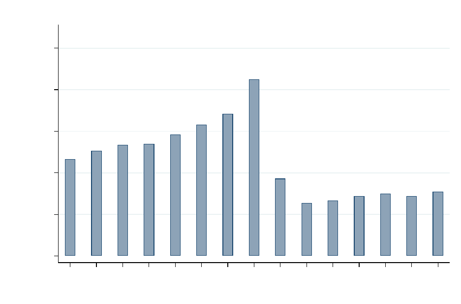
.65
.7
.75
.8
.85
.9
-7 -6 -5 -4 -3 -2 -1 0 1 2 3 4 5 6 7
days around last day of month
Approval rates
Figure 5: The figure shows the average approval rate (approved applications over approved and denied applica-
tions) at the level of the entire United States, for the last eight days of the month, and the first seven days of the fol-
lowing month. The results in the figure are based on the HMDA data from January 1994 to December 2018.
46

0
50
100
150
200
250
percent
-7 -6 -5 -4 -3 -2 -1 0 1 2 3 4 5 6 7
days around last day of month
white Black other race
Number of loans originated (relative to first day of month)
Figure 6: The figure shows average percentage abnormal daily loan origination volume in the U.S., by race group
(whites, Blacks and other races). Abnormal volume is reported for the last eight days of the month, and the first
seven days of the following month, and is computed with respect to loan origination volume on the first day of the
following month, for each group of applicants. The results in the figure are based on the HMDA data from January
1994 to December 2018.
47

-.25
-.2
-.15
-.1
-7 -6 -5 -4 -3 -2 -1 0 1 2 3 4 5 6 7
days around last day of month
Average approval rate gap (Black minus white applications)
(a) Approval Gap (Raw Data)
-.1
-.08
-.06
-.04
-.02
0
residuals
-7 -6 -5 -4 -3 -2 -1 0 1 2 3 4 5 6 7
days around last day of month
Average approval rate gap (Black minus white applications, residuals)
(b) Approval Gap (Residuals)
Figure 7: The figure shows the approval gap for Blacks. Panel (a) reports the difference between the fraction of
approved loans, out of all approved and denied loans in the U.S., for Blacks minus the one for whites, on each of the
last eight days of the month and the first seven days of the following month. Panel (b) reports residual differences
in approval rates after controlling for loan applicant characteristics. The day-by-day difference in approval rates
is attained by first estimating the complete specification of equation 9 (see column 6 of Table 4), but omitting the
dummies for actions taken in the first and last week of the month. We then average regression residuals on each day,
separately for Black and white applicants, and compute the difference between the daily averages to estimate the
(controlled) approval gap on each day. Estimates are based on a 5% sample of the HMDA data from January 1994 to
December 2018.
48

4
4.5
5
5.5
6
6.5
percent
1 2 3 4 5 6 7 8 9 10 11 12 13 14 ... 14 13 12 11 10 9 8 7 6 5 4 3 2 1
days from start of month days from end of month
Share of approved loans by Black applicants out of all loans (by approval date)
(a) United States
2
3
4
5
6
7
8
9
10
11
percent
1 2 3 4 5 6 7 8 9 10 11 12 13 14 ... 14 13 12 11 10 9 8 7 6 5 4 3 2 1
days from start of month days from end of month
median 25-75 percentile range
Distribution of lender approval shares (Black applicants out of all loans)
(b) Individual Lenders
Figure 8: Panel (a) of the figure shows the share of approved applications from Black applicants, out of all ap-
proved applications on each day in the two weeks before and after the end of the month in the United States. The
results in this panel are based on a 5% random sample of the HMDA data from January 1994 to December 2018.
Panel (b) shows the distribution (median, 25th percentile and 75th percentile) of the share of approved applications
from Blacks at the lender level on each day, for all lenders that originate on average at least 10 loans per-day. The
results in this panel are based on the whole HMDA sample from January 1994 to December 2018.
49

0
100
200
300
400
-7 -6 -5 -4 -3 -2 -1 0 1 2 3 4 5 6 7
days around last day of month
prime subprime
Number of loans originated to Black applicants (% relative to first day of month)
(a) Effects for Prime/Subprime Black Applicants
0
50
100
150
200
250
percent
-7 -6 -5 -4 -3 -2 -1 0 1 2 3 4 5 6 7
days around last day of month
1st income quartile 2nd income quartile
3rd income quartile 4th income quartile
Number of loans originated to Black applicants (relative to first day of month)
(b) Effects by Income Quartile Black Applicants
Figure 9: Panel (a) of the figure shows average percentage abnormal daily loan origination volume in the U.S., for
Blacks with prime (660 or higher) and subprime FICO. Abnormal volume is reported for the last eight days of the
month, and the first seven days of the following month, and is computed with respect to loan origination volume on
the first day of the following month for each applicant group. Estimates are based on the merged sample of HMDA
and Black Knight McDash data from 1994 to 2018. Panel (b) of the figure shows average percentage abnormal daily
loan origination volume separately for Blacks belonging to different income quartiles within county. The results in
this panel are based on the HMDA sample from January 1994 to December 2018.
50

0
100
200
300
400
-7 -6 -5 -4 -3 -2 -1 0 1 2 3 4 5 6 7
days around last day of month
prime subprime
Number of loans originated to white applicants (% relative to first day of month)
(a) Effects for Prime/Subprime White Applicants
0
50
100
150
200
percent
-7 -6 -5 -4 -3 -2 -1 0 1 2 3 4 5 6 7
days around last day of month
1st income quartile 2nd income quartile
3rd income quartile 4th income quartile
Number of loans originated to white applicants (relative to first day of month)
(b) Effects by Income Quartile White Applicants
Figure 10: Panel (a) of the figure shows average percentage abnormal daily loan origination volume in the U.S.,
for whites with prime (660 or higher) and subprime FICO. Abnormal volume is reported for the last eight days of the
month, and the first seven days of the following month, and is computed with respect to loan origination volume on
the first day of the following month for each applicant group. Estimates are based on the merged sample of HMDA
and Black Knight McDash data from 1994 to 2018. Panel (b) of the figure shows average percentage abnormal daily
loan origination volume separately for Blacks belonging to different income quartiles within county. The results in
this panel are based on the HMDA sample from January 1994 to December 2018.
51

Tables
Panel (a): Statistics by Year
Year Apps Number Orig Number Loan Amount Lenders Average Orig Number Average Loan Size
(Millions) (Millions) ($ Billions) Number Per Lender ($ 1,000)
1994 12.22 8.25 774.16 9876 835.62 93.81
1995 11.22 7.15 648.27 9544 748.90 90.70
1996 14.42 8.61 799.96 9333 922.24 92.94
1997 15.56 8.78 876.75 7931 1106.87 99.87
1998 23.24 13.75 1531.01 7846 1752.67 111.33
1999 21.71 11.68 1315.98 7824 1492.54 112.69
2000 18.42 9.37 1084.18 7705 1215.83 115.73
2001 23.87 13.69 1856.97 7628 1794.62 135.65
2002 29.06 18.12 2739.76 7780 2329.56 151.17
2003 37.26 23.65 3736.00 8117 2913.08 158.00
2004 30.41 16.41 2782.34 8864 1851.35 169.55
2005 32.13 16.78 3077.99 8859 1894.14 183.43
2006 29.28 15.03 2792.80 8893 1689.79 185.85
2007 23.84 12.00 2359.11 8632 1389.98 196.62
2008 16.15 8.16 1617.75 8418 969.82 198.16
2009 15.91 9.34 1903.12 8148 1146.43 203.74
2010 13.52 8.14 1701.14 7929 1026.50 209.01
2011 12.38 7.43 1563.70 7677 968.46 210.32
2012 16.24 10.37 2266.83 7429 1396.37 218.52
2013 15.19 9.52 2086.19 7201 1322.66 219.03
2014 10.12 5.98 1386.26 7050 848.17 231.83
2015 12.27 7.40 1847.68 6907 1071.99 249.54
2016 14.10 8.38 2180.81 6756 1240.07 260.31
2017 12.23 7.36 2042.92 5860 1255.25 277.73
2018 13.12 7.72 1985.78 5678 1359.87 257.18
Panel (b): Statistics by Applicant Race (1994:2018)
Race Share Average Loan Share Low Share Share Primary Share New Approval Share of
of Applications Amount ($ 1,000) Income Apps Conforming Residence Purchases Rate Approved Loans
White 66.95% 156.21 46.03% 87.24% 91.08% 41.64% 80.72% 73.72%
Black 7.34% 125.12 59.75% 89.23% 91.40% 42.73% 63.25% 5.73%
Other Race 25.71% 176.69 47.80% 87.09% 90.25% 32.95% 69.00% 20.55%
Table 1: Summary statistics for the HMDA loan applications data, covering the whole United States. Panel (a) re-
ports statistics for each year from 1994 to 2018. Panel (b) reports statistics by groups based on applicant race. In
panel (b), Share of Applications is the share of applications belonging to each group out of the total, Share Low In-
come Apps is the fraction of applicants with income below the median in the county and year of the application,
within each group, Share Conforming is the fraction of conforming loans, within each group, Share Primary Resi-
dence is the fraction of loans for which the collateral is the primary residence of the applicant, within each group,
Share New Purchases is the fraction of loans for new house purchase, within each group, Approval Rate is the frac-
tion of approved loans, within each group, and Share of Approved Loans is the fraction of approved loans belonging
to each group of applicants, out of the total.
52

U.S.-Level
(1) (2) (3) (4) (5) (6)
log(Num Loans) log(Num Loans) log(Num Loans) log($ Amount) log(Num Loans) log(Num Loans)
CRA non-CRA
lastweek 0.25*** 0.31*** 0.31*** 0.36*** 0.18*** 0.36***
(0.052) (0.016) (0.012) (0.013) (0.013) (0.013)
firstweek -0.22*** -0.15*** -0.15*** -0.14*** -0.11*** -0.18***
(0.052) (0.016) (0.012) (0.013) (0.013) (0.013)
Holiday FE NO YES YES YES YES YES
Day-of-Week FE NO YES YES YES YES YES
Month FE NO YES NO NO NO NO
Month-Year FE NO NO YES YES YES YES
last − f irst 0.47 0.46 0.46 0.50 0.29 0.54
p − value 0.0000 0.0000 0.0000 0.0000 0.0000 0.0000
N 9131 9131 9131 9131 9131 9131
r2 0.0064 0.91 0.95 0.95 0.95 0.94
Table 2: The table reports regression estimates of the abnormal loan originations volume in the last and first week
of the month (see equation 6). In columns (1) to (3) the dependent variable is the log of the number of originations
per day in the United States. In column (4), the dependent variable is the total dollar amount of loan originations per
day in the United States. In columns (5) and (6) the dependent variable is the log number of originations, respec-
tively, for lenders subject to CRA examination and not subject to CRA examination. lastweek and firstweek are
dummies equal to one, respectively, in the first and last week of the month. The different columns present estimates
based on different choices of lender and seasonality fixed effects. Estimates are based on the sample of HMDA mort-
gage originations from 1994 to 2018.
53

(1) (2) (3) (4) (5) (6) (7) (8) (9) (10) (11) (12) (13)
All Male White Black Other Race Income > Med Income ≤ Med Income Q1 Income Q2 Income Q3 Income Q4 Loan > Med Loan ≤ Med
lastweek 0.029*** 0.028*** 0.026*** 0.050*** 0.028*** 0.024*** 0.034*** 0.038*** 0.031*** 0.026*** 0.023*** 0.031*** 0.028***
(0.00088) (0.00091) (0.00090) (0.0014) (0.00087) (0.00083) (0.0010) (0.0012) (0.0011) (0.00090) (0.00087) (0.0011) (0.00087)
f irstweek -0.016*** -0.016*** -0.016*** -0.025*** -0.016*** -0.015*** -0.019*** -0.021*** -0.019*** -0.016*** -0.013*** -0.018*** -0.017***
(0.0011) (0.0011) (0.0011) (0.0018) (0.0010) (0.00094) (0.0011) (0.0013) (0.0011) (0.00097) (0.00091) (0.00095) (0.0012)
Holiday FE YES YES YES YES YES YES YES YES YES YES YES YES YES
Day-of-Week FE YES YES YES YES YES YES YES YES YES YES YES YES YES
Month-Year FE YES YES YES YES YES YES YES YES YES YES YES YES YES
Lender FE YES YES YES YES YES YES YES YES YES YES YES YES YES
last − f irst 0.045 0.044 0.042 0.076 0.044 0.038 0.052 0.058 0.050 0.043 0.037 0.049 0.045
p − value 0.0000 0.0000 0.0000 0.0000 0.0000 0.0000 0.0000 0.0000 0.0000 0.0000 0.0000 0.0000 0.0000
N 5749198 5468592 5457749 2561526 5711340 5209254 5177984 4496837 4541807 4560944 4509888 5027344 5279720
r2 0.35 0.32 0.32 0.26 0.35 0.32 0.31 0.29 0.28 0.28 0.30 0.32 0.32
Table 3: The table reports regression estimates of abnormal approval rates in the last and first week of the month (see equation 8). The dependent variable is the
approval rate (approval decisions over approval and denial decisions) per day and lender. Column (1) reports results for all applicants, while the other columns
report results for subgroups of applicants based on sex, race, income and loan amount. Income ≤ Med and Loan ≤ Med are income and loan amount smaller
than or equal to the median in the county and year. Income Q1, Income Q2, Income Q3 and Income Q4 are quartiles of the income distribution in each county and
year. lastweek and firstweek are dummies equal to one, respectively, in the first and last week of the month. Standard errors are clustered by lender and year.
Estimates are based on the sample of HMDA mortgage applications and originations from 1994 to 2018.
54

(1) (2) (3) (4) (5) (6)
approval approval approval approval approval approval
Black White & Other All All All All
lastweek 0.090*** 0.057***
(0.0043) (0.0037)
firstweek -0.032*** -0.022***
(0.0028) (0.0025)
black -0.12*** -0.10*** -0.070*** -0.068***
(0.0069) (0.0062) (0.0053) (0.0043)
lastweek 0.057*** 0.048*** 0.044*** 0.043***
(0.0037) (0.0035) (0.0031) (0.0031)
black × lastweek 0.036*** 0.032*** 0.028*** 0.027***
(0.0021) (0.0023) (0.0022) (0.0023)
firstweek -0.022*** -0.021*** -0.019*** -0.020***
(0.0025) (0.0021) (0.0018) (0.0017)
black × firstweek -0.010*** -0.0081*** -0.0073*** -0.0072***
(0.0015) (0.0014) (0.0024) (0.0015)
log(income) 0.095*** 0.073*** 0.071***
(0.0061) (0.0039) (0.0036)
log(loan amount) 0.031*** 0.0089*** 0.0076***
(0.0075) (0.0029) (0.0023)
is conforming 0.13*** 0.092*** 0.090***
(0.0093) (0.0057) (0.0057)
Loan-Level Controls NO NO NO YES YES YES
Holiday FE YES YES YES YES YES YES
Day-of-Week FE YES YES YES YES YES YES
Month-Year FE YES YES YES YES YES NO
County FE YES YES YES YES YES NO
Lender FE NO NO NO NO YES NO
Month-Year-County NO NO NO NO NO YES
Month-Year-Lender NO NO NO NO NO YES
last − f irst 0.12 0.079 0.079 0.068 0.063 0.063
p − value 0.0000 0.0000 0.0000 0.0000 0.0000 0.0000
last − f irst (black) 0.13 0.11 0.099 0.097
p − value (bl ack) 0.0000 0.0000 0.0000 0.0000
last − f irst (black − other) 0.046 0.040 0.035 0.034
p − value (bl ack − other) 0.0000 0.0000 0.0000 0.0000
N 1440405 18200483 19641147 18464497 18463245 17898939
r2 0.050 0.034 0.041 0.092 0.23 0.32
Table 4: The table reports individual loan-level regression estimates of abnormal approval rates in the last and first
week of the month (see equation 9). The dependent variable is a dummy that takes value 1 if a loan application is
approved and 0 if it is denied. lastweek and f irstweek are dummies equal to one, respectively, if the decision on
the application is taken in the first and last week of the month. black is a dummy equal to one for Black applicants.
In columns (1) and (2), the sample is restricted to, respectively, Blacks and whites or other race applicants. The table
also reports estimates of the difference between the coefficients for the dummies lastweek and f irstweek, and
for the difference of the interaction coefficients for Black applicants, along with the p-value of tests of the null that
each difference is equal to 0. Standard errors are clustered by lender and year. Estimates are based on a 5% random
sample of the HMDA data from 1994 to 2018.
55

(1) (2) (3) (4)
Subprime Origination Low Origination
(FICO < 660) LTV (%) Documentation Interest Rate
lastweek 0.00029 0.0062 0.042* 0.00096
(0.00079) (0.070) (0.023) (0.0011)
f irstweek 0.00059 -0.15*** -0.0012 0.00016
(0.00042) (0.028) (0.0012) (0.00094)
black 0.12*** 3.09*** 0.0014 0.0013
(0.0066) (0.24) (0.0034) (0.0019)
black × lastweek 0.0020 -0.32*** -0.018** -0.00076
(0.0014) (0.081) (0.0068) (0.00068)
black × f irstweek 0.0031* 0.098* -0.00042 0.00022
(0.0016) (0.054) (0.0011) (0.00071)
LTV 0.0016*** 0.00032 0.00043
(0.00035) (0.00055) (0.00044)
log(income) -0.011*** -9.02*** 0.013** 0.000068
(0.0039) (0.84) (0.0051) (0.0081)
log(loan amount) -0.041*** 19.8*** -0.028 -0.049***
(0.0061) (1.60) (0.022) (0.012)
is conforming -0.0061** 7.98*** 0.053*** -0.036***
(0.0030) (0.67) (0.012) (0.0062)
FICO 620:659 -1.59*** 0.019 -0.00015
(0.46) (0.025) (0.010)
FICO 660:719 -2.83*** 0.043 -0.020*
(0.56) (0.040) (0.011)
FICO 720:759 -3.99*** 0.051 -0.036***
(0.71) (0.051) (0.011)
FICO 760:799 -7.34*** 0.052 -0.051***
(0.74) (0.054) (0.0099)
FICO ≥ 800 -10.6*** 0.060 -0.065***
(0.67) (0.052) (0.0081)
last − f irst -0.0003 0.1500 0.0430 0.0008
p − value 0.7600 0.0830 0.0690 0.6800
last − f irst (black) -0.0014 -0.2600 0.0250 -0.0002
p − value (black) 0.6100 0.0077 0.1500 0.9100
last − f irst (black − other) -0.0011 -0.4200 -0.0180 -0.0010
p − value (black − other) 0.6600 0.0005 0.0130 0.3700
N 27701585 27701585 18125835 24187005
r2 0.26 0.51 0.51 0.78
Table 5: The table reports regression estimates of the difference in characteristics between mortgages originated
in the last and first week of the month. The dependent variables are a dummy equal to one for subprime loans (with
FICO < 660, see column (1)), the mortgage LTV at origination (column (2)), a dummy equal to one for mortgages
for which the applicant provided low documentation (column (3)), and the mortgage interest rate at origination (col-
umn (4)). lastweek and f irstweek are dummies equal to one in the first and last week of the month. black is a
dummy equal to one for Black applicants. The table also reports estimates of the difference between the coefficients
for the dummies lastweek and f irstweek, and for the difference of the interaction coefficients for Black applicants,
along with their p-values. Standard errors are clustered by lender and year. Estimates are based on the merged sam-
ple of HMDA and Black Knight McDash data from 1994 to 2018.
56

(1) (2) (3) (4) (5)
approval approval approval approval approval
1-30 Days TTA 31-60 Days TTA 61-90 Days TTA > 90 Days TTA
lastweek 0.038*** 0.053*** 0.027*** 0.027*** 0.023***
(0.0026) (0.0033) (0.0031) (0.0030) (0.0034)
firstweek -0.019*** -0.016*** -0.017*** -0.019*** -0.017***
(0.0018) (0.0017) (0.0017) (0.0027) (0.0027)
black -0.056*** -0.072*** -0.043*** -0.037*** -0.030***
(0.0039) (0.0050) (0.0032) (0.0035) (0.0032)
black × lastweek 0.023*** 0.023*** 0.021*** 0.015*** 0.015***
(0.0020) (0.0025) (0.0020) (0.0023) (0.0037)
black × firstweek -0.0094*** -0.0043** -0.015*** -0.0053 -0.0056
(0.0017) (0.0019) (0.0027) (0.0033) (0.0036)
log(TTA) 0.11***
(0.0069)
log(income) 0.058*** 0.083*** 0.038*** 0.040*** 0.036***
(0.0029) (0.0048) (0.0026) (0.0029) (0.0035)
log(loan amount) -0.021*** 0.0022 -0.013*** -0.017*** -0.012***
(0.0026) (0.0029) (0.0020) (0.0026) (0.0035)
is conforming 0.058*** 0.10*** 0.039*** 0.035*** 0.033***
(0.0044) (0.0072) (0.0043) (0.0042) (0.0035)
last − f irst 0.057 0.069 0.044 0.046 0.040
p − value 0.0000 0.0000 0.0000 0.0000 0.0000
last − f irst (black) 0.089 0.096 0.080 0.065 0.061
p − value (bl ack) 0.0000 0.0000 0.0000 0.0000 0.0000
last − f irst (black − other) 0.032 0.027 0.036 0.020 0.021
p − value (bl ack − other) 0.0000 0.0000 0.0000 0.0000 0.0000
N 16503563 9038519 4907587 1420393 1332868
r2 0.35 0.40 0.29 0.37 0.42
Table 6: The table reports individual loan-level regression estimates of abnormal approval rates in the last and first
week of the month (see equation 9), controlling for time to action (TTA), defined as the number of days between
the application date and the date in which action (approval or denial) of the loan is taken. In column (1), the log of
TTA is included as a control. In columns (2) to (5), the sample is restricted to loans with TTA, respectively, between
1 and 30 days, between 31 and 60 days, between 61 and 90 days, and longer than 91 days. The dependent variable
is a dummy that takes value 1 if a loan application is approved and 0 if it is denied. lastweek and f irstweek are
dummies equal to one, respectively, if the decision on the application is taken in the first and last week of the month.
black is a dummy equal to one for Black applicants. The table also reports estimates of the difference between the
coefficients for the dummies lastweek and f irstweek, and for the difference of the interaction coefficients for
Black applicants, along with the p-value of tests of the null that each difference is equal to 0. Standard errors are
clustered by lender and year. Estimates are based on a 5% random sample of the HMDA data from 1994 to 2018.
57

(1) (2) (3) (4)
5-Year Default 5-Year Default 5-Year Default 5-Year Default
FICO < 660 LTV > 80% Low Docs
lastweek -0.00011 -0.00016 -0.00031 0.00042
(0.00027) (0.00047) (0.00033) (0.00077)
f irstweek 0.00044 0.0011 0.00097* 0.00049
(0.00027) (0.00064) (0.00054) (0.00041)
black 0.0033** 0.0011 0.0017 0.0075***
(0.0012) (0.0012) (0.0015) (0.0024)
black × lastweek -0.0013** -0.0020 -0.0022*** -0.0039**
(0.00059) (0.0011) (0.00062) (0.0016)
black × f irstweek 0.0020*** 0.0011 0.0025** 0.0033***
(0.00060) (0.00096) (0.00095) (0.0011)
LTV 0.00032** 0.00049** -0.00016 0.00079**
(0.00012) (0.00018) (0.00030) (0.00033)
log(income) -0.0020 -0.011*** -0.012*** -0.0039**
(0.0016) (0.0036) (0.0022) (0.0016)
log(loan amount) -0.0027 0.0021 0.0061*** 0.0029
(0.0035) (0.0076) (0.0021) (0.0038)
is conforming -0.0037** -0.013*** -0.0075** -0.0051**
(0.0016) (0.0044) (0.0032) (0.0021)
FICO 620:659 -0.0063 -0.0040 -0.013*** 0.0030
(0.0045) (0.0042) (0.0030) (0.0050)
FICO 660:719 -0.020*** -0.026*** -0.014***
(0.0048) (0.0044) (0.0038)
FICO 720:759 -0.029*** -0.035*** -0.028***
(0.0058) (0.0063) (0.0073)
FICO 760:799 -0.033*** -0.040*** -0.034***
(0.0069) (0.0077) (0.0096)
FICO ≥ 800 -0.033*** -0.042*** -0.030***
(0.0072) (0.0082) (0.0089)
last − f irst -0.0006 -0.0012 -0.0013 -0.0001
p − value 0.2800 0.2300 0.1400 0.9400
last − f irst (black) -0.0038 -0.0043 -0.0060 -0.0073
p − value (black) 0.0015 0.0036 0.0023 0.0003
last − f irst (black − other) -0.0033 -0.0031 -0.0047 -0.0072
p − value (black − other) 0.0003 0.0380 0.00080 0.0020
N 20732913 3729582 6606008 5617655
r2 0.12 0.16 0.15 0.22
Table 7: The table reports regression estimates of the difference in performance between mortgages originated in
the last and first week of the month. The dependent variable is a dummy equal to one for mortgages that defaulted
within 5 years after origination. In column (2), the sample is restricted to subprime loans (FICO < 660). In column
(3) the sample is restricted to high loan-to-value loans (LTV> 80%), and in column (4) to loans with low documen-
tation. lastweek and f irstweek are dummies equal to one in the first and last week of the month. black is a dummy
equal to one for Black applicants. The table also reports estimates of the difference between the coefficients for the
dummies lastweek and f irstweek, and for the difference of the interaction coefficients for Black applicants, along
with their p-values. Standard errors are clustered by lender and year. Estimates are based on the merged sample of
HMDA and Black Knight McDash data from 1994 to 2018.
58

(1) (2) (3) (4) (5) (6)
approval approval approval approval approval approval
Fintech Non-Fintech All Shadowbanks No-Shadowbanks All
lastweek 0.064*** 0.036*** 0.035*** 0.034*** 0.053*** 0.054***
(0.011) (0.0030) (0.0031) (0.0037) (0.0081) (0.0081)
f irstweek -0.026*** -0.020*** -0.020*** -0.017*** -0.024*** -0.024***
(0.0045) (0.0034) (0.0034) (0.0030) (0.0037) (0.0037)
black -0.10*** -0.096*** -0.093*** -0.069*** -0.11*** -0.11***
(0.0059) (0.0037) (0.0043) (0.0050) (0.0035) (0.0038)
black × lastweek 0.034*** 0.028*** 0.027*** 0.021*** 0.031*** 0.031***
(0.0038) (0.0037) (0.0034) (0.0040) (0.0034) (0.0035)
black × f irstweek -0.0063* -0.0086*** -0.0074*** -0.0018 -0.0081*** -0.0087***
(0.0033) (0.0023) (0.0024) (0.0043) (0.0025) (0.0024)
black × f intech -0.013
(0.0089)
f intech × lastweek 0.029***
(0.010)
f intech × f irstweek -0.0069
(0.0046)
black × f intech × lastweek 0.0072
(0.0049)
black × f intech × f irstweek 0.00063
(0.0033)
black × shadowbank 0.050***
(0.0076)
shadowbank × lastweek -0.020**
(0.0086)
shadowbank × f irstweek 0.0075*
(0.0042)
black × shadowbank × lastweek -0.0095**
(0.0046)
black × shadowbank × f irstweek 0.0083*
(0.0049)
log(income) 0.075*** 0.077*** 0.077*** 0.058*** 0.082*** 0.077***
(0.0045) (0.0040) (0.0031) (0.0070) (0.0041) (0.0031)
log(loan amount) 0.022*** 0.0016 0.012** -0.011** 0.015*** 0.012***
(0.0055) (0.0036) (0.0042) (0.0048) (0.0040) (0.0039)
is conforming 0.11*** 0.10*** 0.10*** 0.086*** 0.11*** 0.10***
(0.0097) (0.0080) (0.0067) (0.011) (0.0075) (0.0067)
Loan-Level Controls YES YES YES YES YES YES
Holiday FE YES YES YES YES YES YES
Day-of-Week FE YES YES YES YES YES YES
Month-Year-County FE YES YES YES YES YES YES
Month-Year-Lender FE YES YES YES YES YES YES
last − f irst 0.090 0.056 0.050 0.077
p − value 0.0000 0.0000 0.0000 0.0000
last − f irst (black) 0.13 0.092 0.073 0.12
p − value (black) 0.0000 0.0000 0.0000 0.0000
last − f irst (black − other) 0.040 0.037 0.023 0.040
p − value (black − other) 0.0000 0.0000 0.0004 0.0000
last − f irst (black) 0.089 0.12
p − value (black) 0.0000 0.0000
last − f irst (black, Z) 0.096 0.10
p − value (black, Z) 0.0000 0.0000
last − f irst (black, Z − noZ) 0.0066 -0.018
p − value (black, Z − noZ) 0.15 0.022
N 1869937 2172022 4159023 1046528 3195579 4354784
r2 0.26 0.31 0.26 0.42 0.24 0.26
Table 8: The table reports individual loan-level regression estimates of abnormal approval rates in the last and first
week of the month, for lenders with different characteristics (see equation 10). lastweek and firstweek are dum-
mies equal to one, respectively, in the first and last week of the month. black is a dummy equal to one for Black
applicants. In columns (1) and (2) the sample is restricted, respectively, to Fintech and non-Fintech lenders, while
in columns (4) and (5) the sample is restricted to shadow banks and non-shadow banks (deposit-taking institutions).
The table also reports estimates of the difference between the coefficients for the dummies lastweek and f irstweek,
and for the difference of the interaction coefficients for Black applicants across lender groups, along with their p-
values. Standard errors are clustered by lender and year. Estimates are based on a 5% random sample of the HMDA
data from 2014 to 2018.
59

(1) (2) (3) (4) (5) (6)
approval approval approval approval approval approval
High Top4 Sh. Low Top4 Sh. All High HHI Low HHI All
lastweek 0.042*** 0.045*** 0.045*** 0.041*** 0.045*** 0.045***
(0.0031) (0.0031) (0.0030) (0.0031) (0.0031) (0.0030)
f irstweek -0.018*** -0.021*** -0.021*** -0.018*** -0.021*** -0.021***
(0.0015) (0.0019) (0.0019) (0.0015) (0.0019) (0.0019)
black -0.074*** -0.063*** -0.063*** -0.074*** -0.063*** -0.063***
(0.0044) (0.0045) (0.0046) (0.0045) (0.0045) (0.0046)
black × lastweek 0.027*** 0.026*** 0.026*** 0.026*** 0.026*** 0.026***
(0.0024) (0.0022) (0.0022) (0.0023) (0.0023) (0.0023)
black × f irstweek -0.0051** -0.0076*** -0.0079*** -0.0059** -0.0071*** -0.0074***
(0.0021) (0.0015) (0.0015) (0.0022) (0.0015) (0.0014)
black × H(top4) -0.011***
(0.0033)
H(top4) × lastweek -0.0035***
(0.0010)
H(top4) × f irstweek 0.0034***
(0.00088)
black × H(top4) × lastweek 0.0014
(0.0020)
black × H(top4) × f irstweek 0.0027
(0.0020)
black × H(hhi) -0.012***
(0.0033)
H(hhi) × lastweek -0.0040***
(0.0010)
H(hhi) × f irstweek 0.0036***
(0.00084)
black × H(hhi) × lastweek 0.00063
(0.0019)
black × H(hhi) × f irstweek 0.0016
(0.0022)
log(income) 0.071*** 0.069*** 0.071*** 0.072*** 0.069*** 0.071***
(0.0040) (0.0031) (0.0035) (0.0039) (0.0032) (0.0035)
log(loan amount) 0.0075*** 0.0079*** 0.0077*** 0.0078*** 0.0077*** 0.0077***
(0.0022) (0.0025) (0.0023) (0.0022) (0.0025) (0.0023)
is conforming 0.090*** 0.092*** 0.091*** 0.090*** 0.091*** 0.091***
(0.0060) (0.0053) (0.0054) (0.0060) (0.0053) (0.0054)
Loan-Level Controls YES YES YES YES YES YES
Holiday FE YES YES YES YES YES YES
Day-of-Week FE YES YES YES YES YES YES
Month-Year-County FE YES YES YES YES YES YES
Month-Year-Lender FE YES YES YES YES YES YES
last − f irst 0.060 0.066 0.059 0.066
p − value 0.0000 0.0000 0.0000 0.0000
last − f irst (black) 0.092 0.100 0.092 0.100
p − value (black) 0.0000 0.0000 0.0000 0.0000
last − f irst (black − other) 0.032 0.033 0.032 0.033
p − value (black − other) 0.0000 0.0000 0.0000 0.0000
last − f irst (black) 0.100 0.10
p − value (black) 0.0000 0.0000
last − f irst (black, Z) 0.099 0.099
p − value (black, Z) 0.0000 0.0000
last − f irst (black, Z − noZ) -0.0013 -0.0010
p − value (black, Z − noZ) 0.63 0.71
N 8901836 8840521 17898971 8912233 8837435 17898971
r2 0.35 0.30 0.32 0.35 0.30 0.32
Table 9: The table reports individual loan-level regression estimates of abnormal approval rates in the last and first week of the month, for
counties with different concentration of the local mortgage market (see equation 10). lastweek and f irstweek are dummies equal to one, re-
spectively, in the first and last week of the month. black is a dummy equal to one for Black applicants. In columns (1) and (2) the sample is
restricted, respectively, to counties in which the share of the top 4 originators is above and below median (across counties in the United States in
the same year), while in columns (4) and (5) the sample is restricted to counties in which the HHI index based on lenders’ origination shares is
above and below median (across counties in the United States in the same year). The table also reports estimates of the difference between the
coefficients for the dummies lastweek and f irstweek, and for the difference of the interaction coefficients for Black applicants across lender
groups, along with their p-values. Standard errors are clustered by lender and year. Estimates are based on a 5% random sample of the HMDA
data from 1994 to 2018.
60

(1) (2) (3)
approval approval approval
Above Med Size Below Med Size All
lastweek 0.050*** 0.036*** 0.035***
(0.0050) (0.0018) (0.0018)
f irstweek -0.022*** -0.016*** -0.016***
(0.0026) (0.0011) (0.0011)
black -0.070*** -0.064*** -0.064***
(0.0058) (0.0039) (0.0040)
black × lastweek 0.025*** 0.029*** 0.029***
(0.0036) (0.0016) (0.0016)
black × f irstweek -0.0057** -0.0086*** -0.0090***
(0.0025) (0.0016) (0.0015)
black × H(size) -0.0069
(0.0066)
H(size) × lastweek 0.015***
(0.0052)
H(size) × f irstweek -0.0065**
(0.0024)
black × H(size) × lastweek -0.0029
(0.0040)
black × H(size) × f irstweek 0.0034
(0.0030)
log(income) 0.070*** 0.070*** 0.071***
(0.0050) (0.0028) (0.0035)
log(loan amount) 0.0079* 0.0076*** 0.0077***
(0.0040) (0.0023) (0.0023)
is conforming 0.092*** 0.088*** 0.091***
(0.0080) (0.0039) (0.0054)
Loan-Level Controls YES YES YES
Holiday FE YES YES YES
Day-of-Week FE YES YES YES
Month-Year-County FE YES YES YES
Month-Year-Lender FE YES YES YES
last − f irst 0.072 0.052
p − value 0.0000 0.0000
last − f irst (black) 0.10 0.089
p − value (black) 0.0000 0.0000
last − f irst (black − other) 0.031 0.037
p − value (black − other) 0.0000 0.0000
last − f irst (black) 0.089
p − value (black) 0.0000
last − f irst (black, Z) 0.082
p − value (black, Z) 0.0000
last − f irst (black, Z − noZ) -0.0064
p − value (black, Z − noZ) 0.27
N 9172101 8532602 17898971
r2 0.31 0.35 0.32
Table 10: The table reports individual loan-level regression estimates of abnormal approval rates in the last and
first week of the month, for lenders with size (total originated mortgage amount) above and below median (see equa-
tion 10). lastweek and f irstweek are dummies equal to one, respectively, in the first and last week of the month.
black is a dummy equal to one for Black applicants. In columns (1) and (2) the sample is restricted, respectively, to
lenders with size above and below median. The table also reports estimates of the difference between the coefficients
for the dummies lastweek and f irstweek, and for the difference of the interaction coefficients for Black applicants
across lender groups, along with their p-values. Standard errors are clustered by lender and year. Estimates are based
on a 5% sample of the HMDA data from 1994 to 2018.
61
Appendix to:
Using High-Frequency Evaluations to Estimate Discrimination:
Evidence from Mortgage Loan Officers
(intended for online publication)

A.I Identifying Time-Varying Discrimination
We show how under the assumptions in Assumption Set (A) approval probabilities for whites and
Blacks are different. The approval probability, conditional on race and other observable character-
istics, is equal to:
P (a|R, X) =
P (a,R|X)
P (R|X)
=
P (a,R,Z
H
|X)+P (a,Z
L
|X)
P (R|X)
=
P (a|R,Z
H
,X)P (Z
H
|R,X)P (R|X)+P (a|R,Z
L
,X)P (Z
L
|R,X)P (R|X)
P (R|X)
= P (a|Z
H
, R|X)P (Z
H
|R, X) + P (a|Z
L
, R, X)P (Z
L
|R, X)
where Z ∈ {Z
L
, Z
H
} is a binary unobservable characteristic, X is a vector of observable char-
acteristics and R ∈ {W, B} is the applicants’ race (white or Black). Then, the difference in
approval probabilities for whites and Blacks is equal to:
P (a|W, X) − P (a|B, X) =
= [P (a|W, Z
H
, X)P (Z
H
|W, X) + P (a|W, Z
L
, X)P (Z
L
|W, X)] − [P (a|Z
H
, B, X)P (Z
H
|B, X) + P (a|Z
L
, B, X)P (Z
L
|B, X)]
= P (a|Z
H
, X)[P (Z
H
|W, X) − P (Z
H
|B, X)] + P (a|Z
L
, X)[P (Z
L
|W, X) − P (Z
L
|B, X)] > 0
where P (a|Z
H
, X) = P (a|W, Z
H
, X) = P (a|B, Z
H
, X) and P (a|Z
L
, X) = P (a|W, Z
L
, X) =
P (a|B, Z
L
, X) from the assumption of no discrimination, and P (Z
H
|W, X) − P (Z
H
|B, X) > 0
and P (Z
L
|W, X) − P (Z
L
|B, X) < 0 due to the assumption of higher unobservable quality char-
acteristics for whites.
We now turn to the comparison of approval rates for whites and Blacks at the beginning and the
end of the month. The difference in the probability between whites and Blacks is equal to:
P (a|W, X, T ) − P (a|B, X, T ) =
= P (a|Z
H
, W, X, T )P (Z
H
|W, X, T ) + P (a|Z
L
, W, X, T )P (Z
L
|W, X, T ) − P (a|Z
H
, B, X, T )P (Z
H
|B, X, T ) − P (a|Z
L
, B, X, T )P (Z
L
|B, X, T )
= P (a|Z
H
, W, X, T )[P (Z
H
|W, X, T ) − P (Z
H
|B, X, T )] + P (a|Z
L
, W, X, T )[P (Z
L
|W, X, T ) − P (Z
L
|B, X, T )]
= P (a|Z
H
, X, T )[P (Z
H
|W, X, T ) − P (Z
H
|B, X, T )] + P (a|Z
L
, X, T )[P (Z
L
|W, X, T ) − P (Z
L
|B, X, T )]
where T ∈ {Start, End}. Exploiting the calculations above, we can then derive the properties of
the change in difference between approval probabilities at the beginning and the end of the month:
[P (a|W, X, End) − P (a|B, X, End)] − [P (a|W, X, Start) − P (a|B, X, Start)] =
= P (a|Z
H
, X, End)[P (Z
H
|W, X, End) − P (Z
H
|B, X, End)] + P (a|Z
L
, X, End)[P (Z
L
|W, X, End) − P (Z
L
|B, X, End)]
−P (a|Z
H
, X, Start)[P (Z
H
|W, X, Start) − P (X
H
|B, X, Start)] − P (a|Z
L
, X, Start)[P (Z
L
|W, X, Start) − P (Z
L
|B, X, Start)]
ii
= [P (a|Z
H
, X, Start) − P (a|Z
H
, X, Start)][P (Z
H
|W, X) − P (Z
H
|B, X)] + [P (a|Z
L
, X, Start) − P (a|Z
L
, X, Start)][P (Z
L
|W, X) − P (Z
H
|B, X)] = 0
where we set P (Z
H
|W, X, Start) = P (Z
H
|W, X, End) based on the assumption that applica-
tions quality does not change over the month, while P (a|Z
H
, X, T ) = P (a|W, Z
H
, X, T ) =
P (a|B, Z
H
, X, T ) and P (a|Z
L
, X, T ) = P (a|W, Z
L
, X, T ) = P (a|B, Z
L
, X, T ), based on the
no discrimination assumption. Thus, the rejection of the null that the counterpart of the equation
above in the data is equal to zero, leads to a rejection of the no discrimination assumption, con-
ditionally on not having changes in application quality between the beginning and the end of the
month.
iii

A.II Additional Figures and Tables
100
150
200
250
percent
1994 1998 2002 2006 2010 2014 2018
year
Origination volume last week of month divided by first week of month by years
Figure A.1: The figure shows the ratio of average mortgage origination volume in the last week of the month over
average mortgage origination volume in the first week of the month, for each year over the period from 1994 to 2018.
The evidence is based on the HMDA data from January 1994 to December 2018.
iv

-100
0
100
200
300
-7 -6 -5 -4 -3 -2 -1 0 1 2 3 4 5 6 7
Loan volume originated (percentage relative to first day of month)
January December
Figure A.2: The figure shows average percentage abnormal daily loan origination volume (measured as number
of originations) in the U.S., for the last eight days of the month, and the first seven days of the following month,
separately for each calendar month (January to December) over the sample period from January 1994 to December
2018. Abnormal volume is computed with respect to loan origination volume on the first day of the following month.
The evidence is based on the HMDA data from January 1994 to December 2018.
v

-2
-1
0
1
standard deviation
1 2 3 4 5 6 7 8 9 10 11 12 13 14 ... 14 13 12 11 10 9 8 7 6 5 4 3 2 1
days from start of month days from end of month
Loan inventory within month (standardized)
Figure A.3: This figure shows the within-month fluctuation, at the level of the entire United States, in the average
number of loan applications in inventory (awaiting a decision by loan officers) by day of the month. Inventory size
is standardized to have mean of zero and standard deviation of one. The evidence is based on the HMDA data from
January 1994 to December 2018.
vi

Approval Gap Dif. (95% CI)FinTech Lenders Not FinTech Lenders
-.1
0
.1
.2
.3
0
.2
.4
.6
.8
start-of-month end-of-month start-of-month end-of-month FinTech Not FinTech
White Black change in approval gap
Average approval rate
(a) Fintech
Approval Gap Dif. (95% CI)Shadow Bank Not Shadow Bank
-.1
0
.1
.2
.3
0
.2
.4
.6
.8
start-of-month end-of-month start-of-month end-of-month Shadow Bk Not Shadow Bk
White Black change in approval gap
Average approval rate
(b) Shadow banks
Figure A.4: Panel (a) of the figure shows on the left the approval rates for white and Black applicants, in the first
and last week of the month. The rates are shown separately for Fintech and non-Fintech lenders. The right side of
panel (a) shows the change in the approval gap, defined as the difference between the approval rate for white ap-
plicants and the one for Black applicants, between the last and first week of the month, separately for Fintech and
non-Fintech lenders. Panel (b) of the figure shows on the left the approval rates, and on the right the change in the
approval gap, for shadow banks and non-shadow banks (depository institutions). Estimates in this figure are based on
a 5% random sample of the HMDA data from 2014 to 2018.
vii

Approval Gap Dif. (95% CI)High Top 4 Share Low Top 4 Share
-.1
0
.1
.2
.3
0
.2
.4
.6
.8
start-of-month end-of-month start-of-month end-of-month High Top 4 Low Top 4
White Black change in approval gap
Average approval rate
(a) Top 4 Share
Approval Gap Dif. (95% CI)High HHI Low HHI
-.1
0
.1
.2
.3
0
.2
.4
.6
.8
start-of-month end-of-month start-of-month end-of-month High HHI Low HHI
White Black change in approval gap
Average approval rate
(b) HHI
Figure A.5: Panel (a) of the figure shows on the left the approval rates for white and Black applicants, in the first
and last week of the month. The rates are shown separately for counties in which the share of the top 4 lenders is
above and below the median (in the year). The right side of panel (a) shows the approval gap, defined as the differ-
ence between the approval rate for white applicants and the one for Black applicants, between the last and first week
of the month, separately for counties with above and below median top 4 share. Panel (b) of the figure shows on the
left the approval rates, and on the right the change in the approval gap, for counties with Herfindahl-Hirschman Index
(HHI) above and below the median (in the year). Estimates in this figure are based on a 5% random sample of the
HMDA data from 1994 to 2018.
viii

Approval Gap Dif. (95% CI)Lender Size, Above Median Lender Size, Below Median
-.1
0
.1
.2
.3
0
.2
.4
.6
.8
start-of-month end-of-month start-of-month end-of-month Above Below
White Black change in approval gap
Average approval rate
Figure A.6: The figure shows on the left the approval rates for white and Black applicants, in the first and last
week of the month. The rates are shown separately for lenders above and below median size (for each year across
the United States), measured as the total volume of loans originated per year. The right side of the figure shows the
change in the approval gap, defined as the difference between the approval rate for white applicants and the one for
Black applicants, between the last and first week of the month, separately for lenders above and below median size.
Estimates in this figure are based on a 5% random sample of the HMDA data from 1994 to 2018.
ix

U.S.-Level
(1) (2) (3) (4) (5) (6) (7) (8) (9) (10) (11) (12) (13) (14) (15)
White Black Other White Inc Q1 White Inc Q2 White Inc Q3 White Inc Q4 Black Inc Q1 Black Inc Q2 Black Inc Q3 Black Inc Q4 Other Inc Q1 Other Inc Q2 Other Inc Q3 Other Inc Q4
lastweek 0.30*** 0.38*** 0.31*** 0.31*** 0.31*** 0.29*** 0.26*** 0.35*** 0.38*** 0.37*** 0.33*** 0.31*** 0.32*** 0.30*** 0.27***
(0.012) (0.013) (0.012) (0.012) (0.012) (0.012) (0.012) (0.012) (0.013) (0.013) (0.012) (0.012) (0.012) (0.012) (0.012)
f irstweek -0.15*** -0.19*** -0.15*** -0.15*** -0.16*** -0.16*** -0.13*** -0.16*** -0.18*** -0.17*** -0.16*** -0.16*** -0.17*** -0.16*** -0.13***
(0.012) (0.013) (0.012) (0.012) (0.012) (0.012) (0.012) (0.012) (0.013) (0.013) (0.013) (0.012) (0.012) (0.012) (0.012)
Holiday FE YES YES YES YES YES YES YES YES YES YES YES YES YES YES YES
Day-of-Week FE YES YES YES YES YES YES YES YES YES YES YES YES YES YES YES
Month-Year FE YES YES YES YES YES YES YES YES YES YES YES YES YES YES YES
last − f irst 0.45 0.56 0.46 0.46 0.47 0.45 0.39 0.51 0.55 0.54 0.48 0.47 0.48 0.46 0.40
p − value 0.0000 0.0000 0.0000 0.0000 0.0000 0.0000 0.0000 0.0000 0.0000 0.0000 0.0000 0.0000 0.0000 0.0000 0.0000
N 9131 9131 9131 9131 9131 9131 9131 9131 9131 9131 9131 9131 9131 9131 9131
r2 0.95 0.95 0.95 0.95 0.95 0.95 0.95 0.94 0.94 0.94 0.94 0.95 0.95 0.95 0.95
Table A.1: The table reports regression estimates of the abnormal loan originations volume in the last and first week of the month (see equation 6) for borrowers
of different race and income level. The first three columns report results for white, Black and other race applicants, while the remaining columns show, within
each of the three ethnicity groups, breakdown based on income: first, second, third and fourth quartile of income within the county of the loan application (Inc
Q1, Inc Q2, Inc Q3 and Inc Q4). lastweek and f irstweek are dummies equal to one, respectively, in the first and last week of the month. The dependent variable
is the log of the number of originations for each group, at the U.S. level. Standard errors are clustered by lender and year. Estimates are based on the sample of
HMDA mortgage originations from 1994 to 2018.
x

(1) (2) (3) (4) (5) (6) (7) (8) (9) (10) (11) (12) (13)
All Approvals Male White AFA Other Race Income > Med Income ≤ Med Income Q1 Income Q2 Income Q3 Income Q4 Loan > Med Loan ≤ Med
lastweek 0.024*** 0.023*** 0.021*** 0.049*** 0.023*** 0.019*** 0.030*** 0.035*** 0.028*** 0.022*** 0.018*** 0.026*** 0.022***
(0.0012) (0.0012) (0.0012) (0.0020) (0.0011) (0.0012) (0.0014) (0.0016) (0.0014) (0.0012) (0.0012) (0.0015) (0.0012)
f irstweek -0.013*** -0.013*** -0.013*** -0.020*** -0.013*** -0.011*** -0.017*** -0.018*** -0.016*** -0.014*** -0.010*** -0.015*** -0.013***
(0.0012) (0.0013) (0.0013) (0.0023) (0.0012) (0.0012) (0.0014) (0.0016) (0.0015) (0.0012) (0.0012) (0.0012) (0.0014)
CRA month -0.0012 -0.00069 -0.000057 0.0023 -0.0014 -0.0012 -0.00036 -0.000051 -0.00031 -0.00090 -0.000022 -0.00070 -0.0016
(0.0011) (0.00093) (0.00081) (0.0022) (0.0011) (0.0012) (0.0017) (0.0020) (0.0015) (0.0014) (0.0010) (0.00068) (0.0015)
CRA month(+1) -0.00032 -0.00043 0.00056 0.0032 -0.00028 -0.00014 -0.000019 0.000085 -0.00029 -0.00022 0.00020 0.00014 -0.00059
(0.0013) (0.0011) (0.00095) (0.0023) (0.0014) (0.0010) (0.0013) (0.0016) (0.0014) (0.0014) (0.0010) (0.0013) (0.0013)
CRA month(+2) -0.00049 -0.00042 -0.00050 -0.0013 -0.00079 -0.00018 -0.00098 -0.0019 -0.00020 -0.00090 -0.00034 0.000098 -0.0014
(0.0013) (0.0012) (0.0012) (0.0028) (0.0012) (0.0014) (0.0016) (0.0019) (0.0014) (0.0020) (0.0012) (0.0010) (0.0017)
CRA month(+3) -0.0023* -0.0021 -0.0018 0.00039 -0.0020 -0.0018* -0.0017 0.0011 -0.0030 -0.00064 -0.0011** -0.00067 -0.0016
(0.0013) (0.0013) (0.0011) (0.0024) (0.0013) (0.0010) (0.0020) (0.0024) (0.0018) (0.0017) (0.00049) (0.0011) (0.0019)
CRA month(-1) -0.0020** -0.0016 -0.0012* -0.0022 -0.0017** -0.0013 -0.0020* -0.0019 -0.0019 -0.0014 -0.0015** -0.0018* -0.0020*
(0.00071) (0.00098) (0.00057) (0.0028) (0.00069) (0.00080) (0.0010) (0.0014) (0.0018) (0.0011) (0.00064) (0.00098) (0.00096)
CRA month(-2) -0.0011 -0.0015* -0.00075 0.0021 -0.0010 -0.00099 -0.00059 0.00074 -0.0015 -0.00092 -0.00030 -0.00068 -0.0015
(0.00088) (0.00083) (0.00081) (0.0028) (0.00090) (0.00100) (0.0014) (0.0017) (0.0019) (0.0013) (0.0010) (0.0011) (0.0013)
CRA month(-3) -0.00074 -0.0010 -0.00076 -0.0013 -0.00063 -0.00065 -0.00088 -0.00062 -0.0021 -0.0019 0.00040 0.00027 -0.0014
(0.0010) (0.00098) (0.00091) (0.0025) (0.0011) (0.00085) (0.0016) (0.0017) (0.0018) (0.0012) (0.0011) (0.00065) (0.0012)
Holiday FE YES YES YES YES YES YES YES YES YES YES YES YES YES
Day-of-Week FE YES YES YES YES YES YES YES YES YES YES YES YES YES
Month-Year FE YES YES YES YES YES YES YES YES YES YES YES YES YES
Lender FE YES YES YES YES YES YES YES YES YES YES YES YES YES
N 2216169 2116758 2122995 823391 2205077 2020223 1976495 1711880 1694957 1717338 1779768 1878114 2049297
r2 0.25 0.22 0.22 0.16 0.25 0.22 0.21 0.19 0.19 0.19 0.20 0.22 0.22
Table A.2: The table reports regression estimates of abnormal approval rates in the last and first week of the month. The dependent variable is the approval rate
(approval decisions over approval and denial decisions) per day and lender. Column (1) reports results for all applicants, while the other columns report results
for subgroup of applicants based on sex, race, income and loan amount. Income ≤ Med and Loan ≤ Med are income and loan amount smaller than or equal to the
median in the county and year. Income Q1, Income Q2, Income Q3 and Income Q4 are quartiles of the income distribution in each county and year. lastweek and
firstweek are dummies equal to one, respectively, in the first and last week of the month. We include controls accounting for whether the lender is subject to a
CRA examination in the current month, or the previous or next three months. Estimates are based on the sample of HMDA mortgage applications and originations
from 1994 to 2018.
xi

(1) (2) (3) (4) (5) (6) (7)
approval approval approval approval approval approval approval
All All New Purchases Refinancing Conforming All
lastweek 0.043*** 0.043*** 0.035*** 0.051*** 0.043*** 0.043***
(0.0030) (0.0030) (0.0021) (0.0049) (0.0032) (0.0031)
f irstweek -0.020*** -0.020*** -0.014*** -0.025*** -0.020*** -0.019***
(0.0017) (0.0017) (0.0011) (0.0026) (0.0018) (0.0017)
black -0.067*** -0.070*** -0.056*** -0.067*** -0.068*** -0.064***
(0.0043) (0.0036) (0.0059) (0.0043) (0.0044) (0.0043)
black × lastweek 0.027*** 0.027*** 0.028*** 0.025*** 0.026*** 0.028***
(0.0021) (0.0021) (0.0018) (0.0041) (0.0022) (0.0021)
black × f irstweek -0.0074*** -0.0073*** -0.0063*** -0.0096*** -0.0067*** -0.0072***
(0.0015) (0.0015) (0.0015) (0.0024) (0.0015) (0.0015)
f emale -0.017***
(0.0025)
lastday 0.081***
(0.0068)
f irstday -0.020***
(0.0031)
black × lastday 0.046***
(0.0039)
black × f irstday -0.0069**
(0.0033)
log(income) 0.071*** 0.069*** 0.058*** 0.068*** 0.071*** 0.071*** 0.071***
(0.0035) (0.0034) (0.0038) (0.0038) (0.0034) (0.0036) (0.0036)
log(loan amount) 0.0076*** 0.0073*** 0.0031 -0.010* 0.0089*** 0.0077*** 0.0079***
(0.0023) (0.0023) (0.0021) (0.0050) (0.0024) (0.0023) (0.0023)
is conforming 0.090*** 0.090*** 0.058*** 0.084*** 0.091*** 0.091***
(0.0054) (0.0054) (0.0038) (0.0056) (0.0055) (0.0055)
black-Year YES NO NO NO NO NO NO
Loan-Level Controls YES YES YES YES YES YES YES
Holiday FE YES YES YES YES YES YES YES
Day-of-Week FE YES YES YES YES YES YES YES
Lender FE YES YES YES YES YES YES YES
Month-Year-County YES YES YES YES YES YES YES
Month-Year-Lender YES YES YES YES YES YES YES
last − f irst 0.063 0.063 0.049 0.076 0.063 0.062 0.10
p − value 0.0000 0.0000 0.0000 0.0000 0.0000 0.0000 0.0000
last − f irst (black) 0.097 0.097 0.084 0.11 0.096 0.097 0.15
p − value (black) 0.0000 0.0000 0.0000 0.0000 0.0000 0.0000 0.0000
last − f irst (black − other) 0.034 0.034 0.035 0.034 0.033 0.035 0.053
p − value (black − other) 0.0000 0.0000 0.0000 0.0000 0.0000 0.0000 0.0000
N 17898971 17898971 7046904 8705784 16392963 17893870 17893870
r2 0.32 0.32 0.33 0.35 0.32 0.32 0.32
Table A.3: The table reports individual loan-level regression estimates of abnormal approval rates in the last and
first week of the month (see equation 9). The dependent variable is a dummy that takes value 1 if a loan application
is approved and 0 if it is denied. For all columns the regression specification includes all the controls used in column
6 of Table 4. In column (3) the sample is restricting to new mortgages issued for home purchases, in column (4)
it is restricted to refinanced mortgages, and in column (5) to conforming mortgages. Columns (6) and (7) redefine
month fixed effects so that a month breaks at the 15th day. This helps comparing differences in approval rates in
weeks or days immediately adjacent to the calendar month cutoff. lastweek and firstweek are dummies equal to
one, respectively, if the decision on the application is taken in the first and last week of the month, while lastday and
firstday are dummies equal to one, respectively, if the decision on the application is taken in the first and last day
of the month. black is a dummy equal to one for Black applicants and f emale is a dummy equal to one for female
applicants. The table also reports estimates of the difference between the coefficients for the dummies lastweek and
firstweek (lastday and f irstday), and for the difference of the interaction coefficients for Black applicants, along
with the p-value of tests of the null that each difference is equal to 0. Standard errors are clustered by lender and
year. Estimates are based on a 5% random sample of the HMDA data from 1994 to 2018.
xii

(1) (2) (3) (4)
Time to Time to Time to Time to
Origination Origination Denial Action
lastweek -0.49***
(0.15)
f irstweek -0.55***
(0.13)
black 3.08*** -0.85*** 0.76**
(0.39) (0.16) (0.29)
lastweek -0.51*** 0.72*** 0.13
(0.15) (0.12) (0.24)
f irstweek -0.54*** 0.73*** 0.53
(0.13) (0.16) (0.49)
black × lastweek 0.26* 0.13 0.82***
(0.13) (0.13) (0.14)
black × f irstweek -0.26** -0.063 -0.052
(0.11) (0.15) (0.100)
log(income) -1.01*** -0.94*** 1.35*** 0.95***
(0.17) (0.17) (0.12) (0.15)
log(loan amount) 5.38*** 5.41*** 3.16*** 4.56***
(0.31) (0.32) (0.37) (0.31)
is conforming 1.08** 1.10** 1.74*** 1.54***
(0.40) (0.41) (0.32) (0.35)
last − f irst 0.0590 0.0240 -0.0083 -0.4000
p − value 0.7900 0.9100 0.9700 0.3300
last − f irst (black) 0.5400 0.1800 0.4800
p − value (black) 0.02800 0.2900 0.3000
last − f irst (black − other) 0.5200 0.1900 0.8800
p − value (black − other) 0.0031 0.2500 0.0000
N 11924971 11924971 3915189 20683438
r2 0.29 0.29 0.40 0.25
Table A.4: The table reports individual loan-level regression estimates of abnormal mortgage processing time in
the last and first week of the month. We use the same specification as in equation 9. In column (1), the sample is
restricted to applications from Black applicants, while in all other columns the sample includes all applicants. In
columns (1) and (2), the sample is restricted to originated loans, and the dependent variable is the time to origina-
tion, defined as the number of days between the application date and the origination date. In column (3), the sample
is restricted to denied applications, and the dependent variable is the time to denial. In column (4), the sample in-
cludes both approved and denied loans, and the dependent variable is time to action (time to approval). lastweek
and firstweek are dummies equal to one, respectively, if the decision on the application is taken in the first and last
week of the month. black is a dummy equal to one for Black applicants. The table also reports estimates of the dif-
ference between the coefficients for the dummies lastweek and f irstweek, and for the difference of the interaction
coefficients for Black applicants, along with the p-value of tests of the null that each difference is equal to 0. Stan-
dard errors are clustered by lender and year. Estimates are based on a 5% random sample of the HMDA data from
1994 to 2018.
xiii

(1) (2) (3) (4)
5-Year Termination 5-Year Termination 5-Year Termination 5-Year Termination
FICO < 660 LTV > 80% Low Docs
lastweek -0.0026 -0.00060 -0.0041* 0.0023
(0.0022) (0.0012) (0.0020) (0.0038)
f irstweek 0.0010 0.00032 0.0018 -0.00028
(0.0014) (0.0020) (0.0016) (0.0017)
black -0.054*** -0.038*** -0.061*** -0.044***
(0.0083) (0.0063) (0.0091) (0.0086)
black × lastweek -0.0024* -0.0043*** -0.0014 -0.0088**
(0.0014) (0.0012) (0.0015) (0.0039)
black × f irstweek 0.0018 0.0013 0.0033 0.0036**
(0.0018) (0.0019) (0.0021) (0.0014)
LTV -0.0015*** -0.0011*** -0.0029*** -0.0016***
(0.00043) (0.00031) (0.00061) (0.00050)
log(income) 0.025*** 0.0018 0.028*** 0.023**
(0.0073) (0.011) (0.0080) (0.0086)
log(loan amount) 0.096*** 0.068*** 0.12*** 0.11***
(0.018) (0.010) (0.016) (0.021)
is conforming 0.087*** 0.080*** 0.090*** 0.13***
(0.027) (0.011) (0.018) (0.035)
FICO 620:659 0.016 0.024* 0.011 0.0042
(0.013) (0.012) (0.012) (0.0059)
FICO 660:719 0.028 0.030 0.010
(0.020) (0.020) (0.0080)
FICO 720:759 0.039 0.044* 0.034**
(0.025) (0.024) (0.012)
FICO 760:799 0.048 0.051* 0.067***
(0.031) (0.028) (0.017)
FICO ≥ 800 0.032 0.029 0.066***
(0.032) (0.029) (0.018)
last − f irst -0.0036 -0.00092 -0.0059 0.0026
p − value 0.2900 0.7700 0.0780 0.6200
last − f irst (black) -0.0078 -0.0066 -0.0110 -0.0099
p − value (black) 0.1100 0.0440 0.0067 0.1200
last − f irst (black − other) -0.0042 -0.0057 -0.0047 -0.0120
p − value (black − other) 0.1200 0.0410 0.1000 0.0047
N 20732913 3729582 6606008 5617655
r2 0.22 0.28 0.25 0.32
Table A.5: The table reports regression estimates of the difference in performance between mortgages originated
in the last and first week of the month. The dependent variable is a dummy equal to one for mortgages that were
terminated (due to default or refinancing) within 5 years after origination. In column (2), the sample is restricted to
subprime loans (FICO < 660). In column (3) the sample is restricted to high loan-to-value loans (LTV> 80%),
and in column (4) to loans with low documentation. lastweek and firstweek are dummies equal to one in the first
and last week of the month. black is a dummy equal to one for Black applicants. The table also reports estimates
of the difference between the coefficients for the dummies lastweek and f irstweek, and for the difference of the
interaction coefficients for Black applicants, along with their p-values. Standard errors are clustered by lender and
year. Estimates are based on the merged sample of HMDA and Black Knight McDash data from 1994 to 2018.
xiv
